 Learn About Structures
The cantilever method is very similar to the portal method. We still put hinges at the middles of the beams and columns. The only difference is that for the cantilever method, instead of finding the shears in the columns first using an assumption, we will find the axial force in the columns using an assumption.
The assumption that is used to find the column axial force is that the entire frame will deform laterally like a single vertical cantilever. This concept is shown in Figure 7.8. When a cantilever deforms laterally, it has a strain profile through its thickness where one face of the cantilever is in tension and the opposite face is in compression, as shown in the top right of the figure. Since we can generally assume that plain sections remain plane (see Chapter 5), the strain profile is linear as shown. The relative values of the tension and compression strain are dependant on the location of the neutral axis for bending, which is in turn dependant on the shape of the cantilever's cross-section.
The cantilever method assumed that the whole frame will deform laterally in the same way as the vertical cantilever. The location of the neutral axis of the whole frame is found by considering the cross-sectional areas and locations of the columns at each storey:
\begin{equation} \boxed { \bar{x}= \frac{\sum_i (A_{i} x_{i})}{\sum_i A_{i}} } \label{eq:frame-neutral-axis} \tag{1}\end{equation}
where $\bar{x}$ is the horizontal distance between the location of the neutral axis and the zero point, $A_{i}$ is the area of column $i$, and $x_i$ is the horizontal distance between column $i$ and the zero point. The location zero does not matter, but is commonly set as the location of the leftmost column.
Once we know the location of the neutral axis, using the assumption that the frame behaves as a vertical cantilever, we know that the axial strain in each column will be proportional to that column's distance from the neutral axis, just like the strain in any fibre a distance $x$ away from the neutral axis of a cantilever is proportional to the distance $x$. Since we are assuming that all of our materials are linear (stress is linear to strain), then this also means that the axial stress in each column is proportional to it's distance from the neutral axis of the frame. Also, columns on one side of the neutral axis will be in tension, and columns on the other side of the neutral axis will be in compression. The linear axial stress profile for a sample structure is shown at the bottom of Figure 7.8. If we assume an unknown value for the stress in the left column ($\sigma_1$ in the figure) then the cantilever method can be used to find the stress in the other two columns as a function of their relative distance from the neutral axis as shown in the figure. From these relative stresses, we can determine the force in each column as a function of stress $\sigma_1$. Then, using a global moment equilibrium, we can solve for $\sigma_1$, and therefore for the axial force in each column. From this point, the structure is again broken into separate free body diagrams between the hinges as was done for the portal method and all of the remaining unknown forces at the hinges are found using equilibrium.
Since this method relies on the frame behaving like a bending cantilevered beam, it should generally be more accurate for more slender or taller structures, whereas the portal method may be more accurate for shear critical frames, such as squat or short structures.
Example
The details of the cantilever method process will be illustrated using the same example structure that was used for the portal method (previously shown in Figure 7.4).
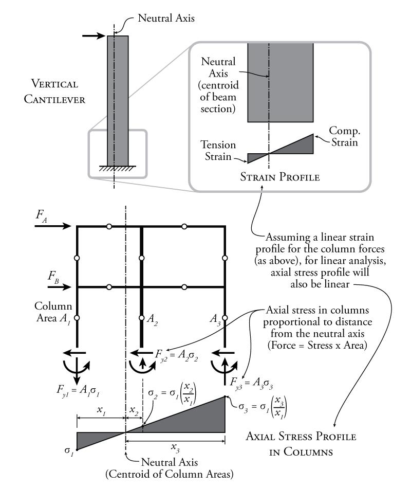
The most important part of the cantilever method analysis is to find the axial forces in the columns at each storey. We will start with the top story as shown at the top of Figure 7.9.
First, we must find the location of the neutral axis for the frame when cut at the top story using equation \eqref{eq:frame-neutral-axis} (the column cross-sectional areas are the same for both storeys and are shown in Figure 7.4):
\begin{align*} \bar{x} &= \frac{\sum_i (A_{i} x_{i})}{\sum_i x_{i}} \\ \bar{x} &= \frac{{10\,000}(0) + {20\,000}(5) + {15\,000}(10)}{ {10\,000} + {20\,000} + {15\,000}} \\ \bar{x} &= 5.555\mathrm{\,m} \end{align*}
where the location of the left column is selected as the zero point.
Knowing the neutral axis location (as shown in the top diagram of Figure 7.9), we can determine the axial stress in all of the columns in the top storey. We will do this in terms of the stress in the left column, which we will call $\sigma_2$ as shown. The stress in the middle column will be equal to $\sigma_2$ multiplied by the ratio of the distance from the second column to the neutral axis to the distance from the first column to the neutral axis:
\begin{align*} \left( \frac{0.56}{5.56} \right) \sigma_2 = 0.1\sigma_2 \end{align*}
Likewise, the stress in the right column will be:
\begin{align*} \left( \frac{4.44}{5.56} \right) \sigma_2 = 0.8\sigma_2 \end{align*}
From these stresses, we can determine the force in the columns by multiplying the stress in each column by it's cross-sectional area as shown in the top diagram of Figure 7.9. Also, the left and middle columns are on the tension side of the neutral axis, so the column axial force arrows will point down as shown (pulling on the column) and the right column is on the compression side of the neutral axis, so the column axial force arrow for that column will point up as shown.
Now, we can use a moment equilibrium on the top story free body diagram in Figure 7.9 to solve for the unknown stress. We will use the moment around point f:
\begin{align*} \curvearrowleft \sum M_f &= 0 \\ -100\mathrm{\,kN} ( 2\mathrm{\,m} ) - A_{col2} (0.1 \sigma_2) (5\mathrm{\,m}) + A_{col3} (0.8 \sigma_2) (10\mathrm{\,m}) &= 0 \\ -100\mathrm{\,kN} ( 2\mathrm{\,m} ) - (0.02\mathrm{\,m^2}) (0.1 \sigma_2) (5\mathrm{\,m}) + (0.015\mathrm{\,m^2}) (0.8 \sigma_2) (10\mathrm{\,m}) &= 0 \\ \sigma_2 = 1818.2\mathrm{\,kN/m^2}& \end{align*}
This resulting stress in the left column may be subbed back into the equations for the force in each column shown in the figure to get forces of $18.2\mathrm{\,kN}\downarrow$ in the left column, $3.6\mathrm{\,kN}\downarrow$ in the middle column, and $21.8\mathrm{\,kN}\uparrow$ in the right column.
For the lower story, the column areas are the same, so the neutral axis will be located in the same place as shown in the lower diagram in Figure 7.9. This means that the relative stresses will also be the same. To solve for the stresses in the left column again for the lower storey ($\sigma_1$), we need to take a free body diagram of the entire structure above the hinge in the middle of the lower column (as shown in the figure). We should cut the lower storey at the hinge location because that way we do not have any moments at the cut (since the hinge is, by definition, a location with zero moment). If we chose to cut the structure at the base of the columns instead, we would have additional point moment reaction at the base of each column which would have to be considered in the moment equilibrium (which are unknown). Such moment reactions at the base of the columns are shown in Figure 7.8. These extra moments would make it impossible to solve the equilibrium equation for $\sigma_1$. So, taking the cut at the lower hinges as shown in the lower diagram in Figure 7.9, we can solve for $\sigma_1$ using a global moment equilibrium about point a:
\begin{align*} \curvearrowleft \sum M_a &= 0 \\ -100(6) - 50(2) - (0.02)(0.1 \sigma_1)(5) + (0.015)(0.8 \sigma_1)(10) &= 0 \\ \sigma_1 = 6363.6\mathrm{\,kN/m^2}& \end{align*}
This resulting stress in the left column may be subbed back into the equations for the force in each column shown in the figure to get forces of $63.6\mathrm{\,kN}\downarrow$ in the left column, $12.7\mathrm{\,kN}\downarrow$ in the middle column, and $76.4\mathrm{\,kN}\uparrow$ in the right column.
From this point forward, the solution method is the same as it was for the portal method. Split each storey free body diagram into separate free body diagrams with cuts at the hinge locations, and then work methodically through using equilibrium to find all of the unknown forces at the hinge cuts. This process is illustrated in Figure 7.10.
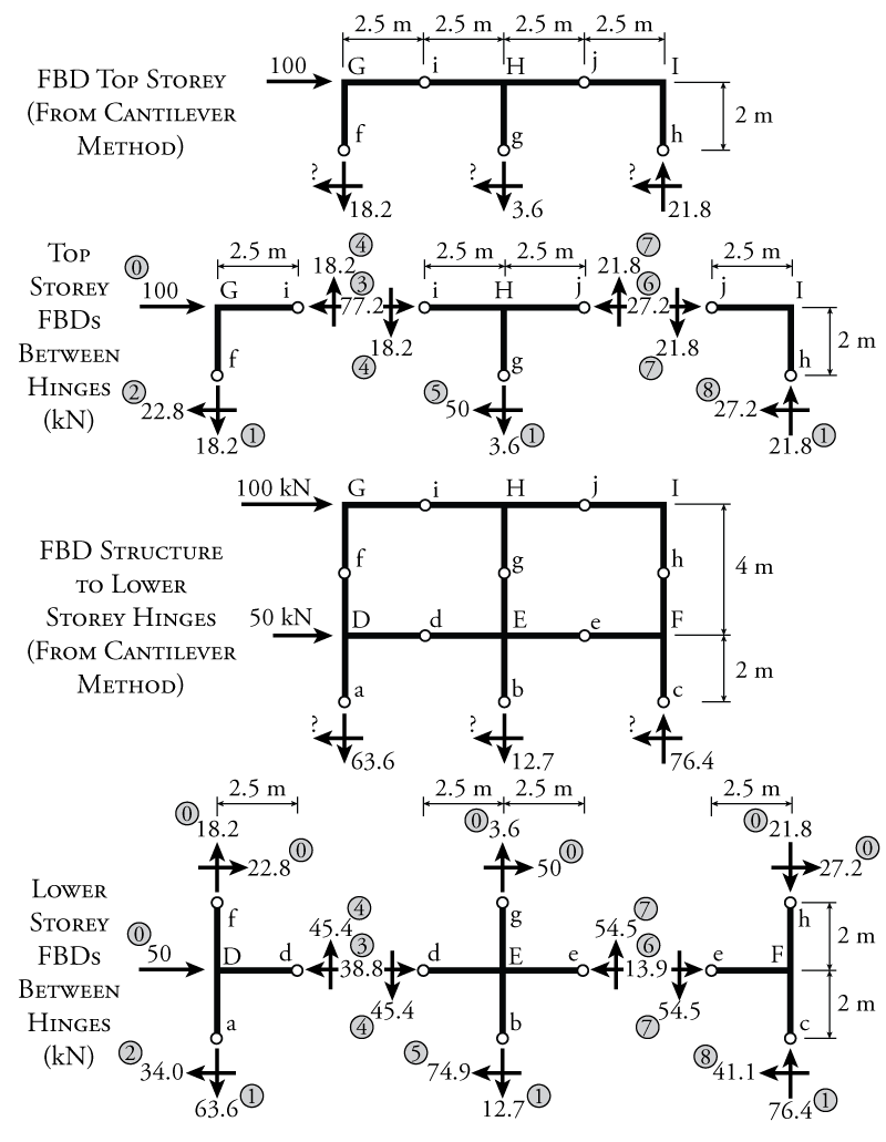
Like the portal frame example, the free body diagrams in Figure 7.10 are annotated with numbers in grey circles to show a suggested order for solving all of the unknown forces. Of course, as before, step 0 and step 1 consist of known values, either caused by external forces or the previous storey (for step 0) or the column axial forces that were solved using the cantilever method assumptions (for step 1). The rest of the unknowns are solved for using vertical, horizontal or moment equilibrium.
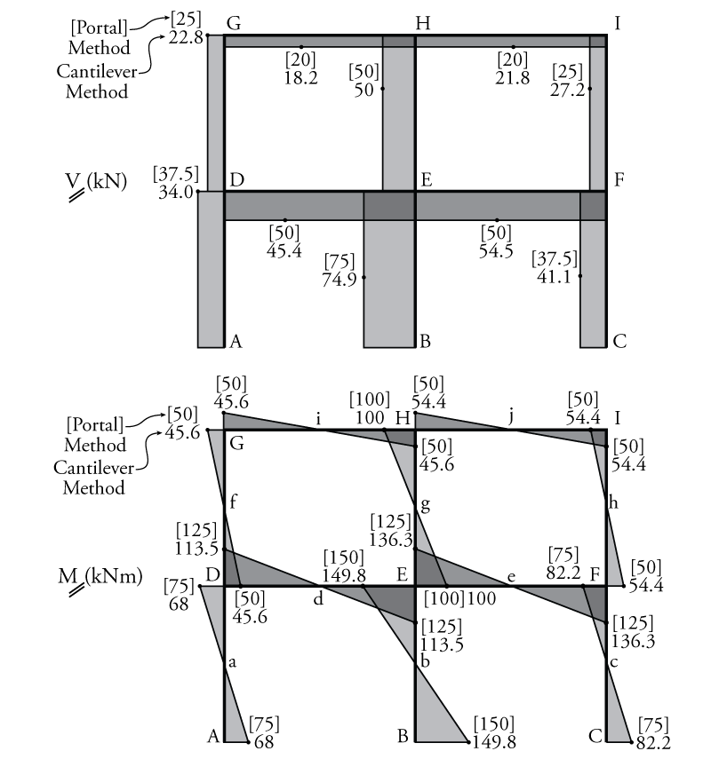
Once all of the unknown forces at the hinges are found, the shear and moment diagrams for the frame may be drawn using the same methods that were used for the previously described portal method analysis example. The final shear and moment diagrams for this analysis are shown in Figure 7.11. This figure shows both the values from this cantilever method analysis compared with the previous portal method analysis example results (in square brackets). This shows that with a significantly different set of assumptions for this example frame, we get similar shear and moment diagrams using the two different methods.