 Learn About Structures
The conjugate beam method provides a different way to find slopes (rotations) and deflections of determinate beams. It takes advantage of the similar set of relationships that exist between load ($w$) - shear ($V$) - moment ($M$) and curvature ($\phi$) - slope ($\theta$) - deflection ($\Delta$). Recall the relationships between load, shear and moment (equations \eqref{eq:shear-int} and \eqref{eq:moment-int} from Section 4.3):
\begin{align} V(x) &= \int w(x) \, dx \label{eq:shear-int} \tag{1} \\ M(x) &= \int V(x) \, dx \label{eq:moment-int} \tag{2} \end{align}
Likewise, recall the relationships between curvature, slope and deflection from equations \eqref{eq:curv-slope} and \eqref{eq:slope-defl}:
\begin{align} \theta(x) &= \int \phi(x) \, dx \label{eq:curv-slope} \tag{3} \\ \Delta(x) &= \int \theta(x) \, dx \label{eq:slope-defl} \tag{4} \end{align}
There is a clear parallel here between the two sets of relationships. This is summarized in Figure 5.9. This figure suggests that, if we could somehow treat the curvature diagram as if it was a loading diagram, then we could determine slope and deflection using graphical integration, the same method that we currently can use to find the shears and moments. This could potentially be an easy way to find the slopes and deflections.
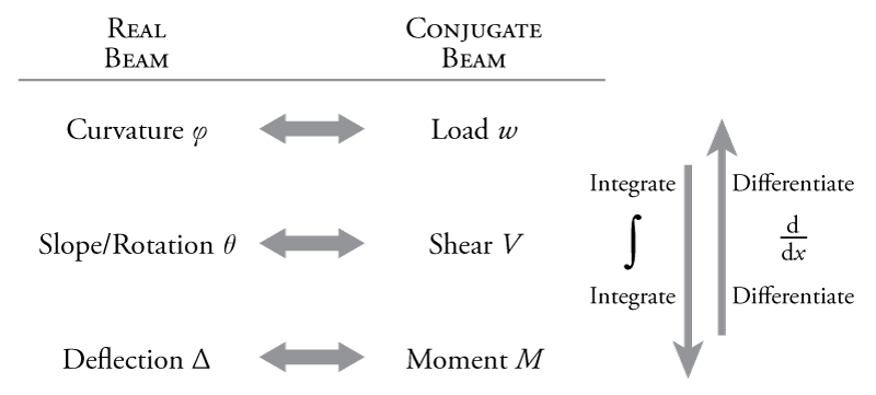
So, let's create a conjugate beam with the same geometry as the real beam but treating the curvatures as the loads. In this new conjugate beam, the 'shears' would actually be the slopes of the real beam and the 'moments' would actually be the deflections of the real beam (using the relationships shown in Figure 5.9). It sounds easy, but there is one problem: if in this beam the conjugate shears represent the real slopes and the conjugate moments represent the real deflections, then we also need to convert our boundary conditions so that they have the same effect on the shear and moment in the conjugate beam as the boundary conditions had on the slope and deflection in the real beam. This conversion process for the supports in conjugate beams is shown in Figure 5.10.
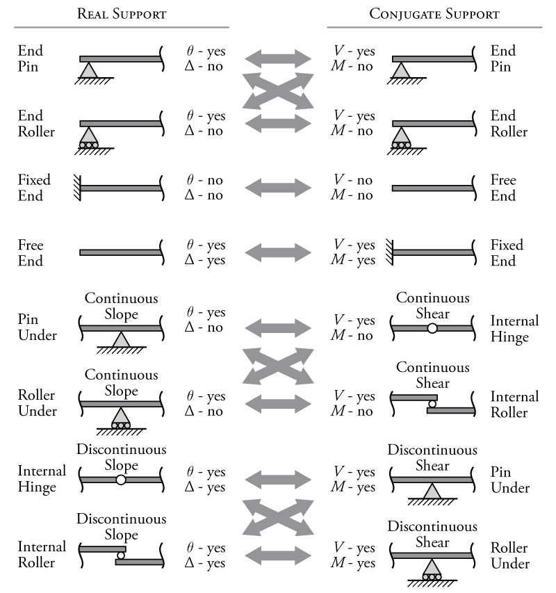
Figure 5.10 shows the equivalent conjugate supports for each given real support. For example, a fixed end in a real beam restrains both rotation and deflection ($\Delta$ and $\theta$ both equal zero at a fixed support). Therefore, for the equivalent conjugate support we need a support that has zero shear (equivalent to zero rotation in the real beam) and zero moment (equivalent to zero deflection in the real beam). The only support that fits these requirements is no support (a free end). So, any fixed support in in real beam will be replaced with a free end in the conjugate beam.
Likewise, pins and rollers at the end of a real beam allow rotation ($\theta \neq 0$) but restrain deflection ($\Delta = 0$). Therefore, for the equivalent conjugate support we need a support that allows a non-zero shear (it provides a vertical reaction) but has zero moment (does not have a moment reaction component). A pin or roller also happens to satisfy these requirements. So, the conjugate support for a pin or roller in the real beam, is a pin or roller. Note that it doesn't matter whether you choose a beam or a roller from the beam's point of view because for beam problems, we typically do not consider axial loads.
For internal supports or supports underneath a beam, pins (or hinges) and rollers are also interchangeable, as they were at the ends of beams; however, support conditions which are not at the end of a beam are a bit more complex because we must consider how the slope and shear change at the support location, not only if one exists. For a pin under a beam, it allows rotation, but no deflection, and the slope of the beam is continuous (there is no 'kink' in the beam shape). This means that in the conjugate beam at the same location, there should be a shear in the beam but no moment and the shear should be continuous (it should not step). Recall that steps in the shear force diagram are caused by point loads or point reactions, so this means that there should be no support reaction at that location on the conjugate beam. An internal hinge satisfies all these requirements, it transfers shear but not moment, and it has no external support reaction associated with it, so the shear diagram will be continuous at that location.
For an internal hinge in the real beam, the reverse case is true. It allows rotation and deflection (it can move up or down since there is no vertical support reaction). It also allows a discontinuous slope at the hinge location, i.e. the beam can have a 'kink' and the hinge, meaning that the tangent slope of the beam is different on either side of the hinge. Therefore, the conjugate support must have both shear and moment and must have a discontinuous shear at that location on the beam. A continuous beam with a pin support satisfies these criteria. The continuity of the beam allows the transfer of shear and moment, and the support reaction provided by the pin causes a step in the shear diagram at that location (a discontinuity in the shear).
Some example conversions from real beams to conjugate beams are shown in Figure 5.11. Notice from these that if the real beam is determinate, then the conjugate beam will also be determinate; however, if the real beam is indeterminate, then the conjugate beam will be unstable, and vice versa. This method is most useful for calculating the slopes and deflections of determinate structures.

Example
The conjugate beam method analysis will be illustrated using the example beam shown in Figure 5.12.

The beam shown in Figure 5.12 is a simple propped cantilever with a single point load and a point moment at the end. This beam is determinate and may easily be analysed using the methods from Section 4.3. The most difficult part about this analysis is finding the reactions in the first step. This may be done by first analysing a free body diagram of member CD to find the reaction $C_y$ and shear at the hinge (remembering that the moment at C must be zero due to the presence of the hinge). Then a free body diagram of AC can be used together with the carried-over hinge shear to find the rest of the unknown reactions. The completed shear and moment diagrams for the beam are shown in the figure just below the beam. Notice that the moment diagram is zero at the location of the hinge as expected. Since the cross-section and material for this beam are constant ($EI$ is constant), the curvature diagram ($\phi$) is simply the moment diagram divide by $EI$. This curvature diagram is shown directly below the moment diagram.
Now that we have constructed the curvature diagram, we can form the conjugate beam (which is shown below the curvature diagram). In the conjugate beam, the curvatures from the curvature diagram of the real beam are treated as distributed loads and the support conditions are converted as discussed in the previous section and shown in Figure 5.10. Therefore, the fixed end at A becomes a free end, the hinge at C becomes a pin support below the beam at that point, and the end roller at point D remains a roller.
The first step in the analysis of the conjugate beam is to determine the reaction 'forces' (which are actually curvatures) using global equilibrium. The resulting reaction forces are shown on the free body diagram (FBD) of the composite beam in Figure 5.12.
Now, treating the curvatures as distributed forces, we can construct the conjugate `shear force diagram' using the methods from Section 4.3. This diagram will actually give us the slopes of the real beam. In this process, we must consider the area under the 'distributed load', jumps in the 'shear' due to the reactions, and the appropriate slope of each point on the 'shear diagram' (which is equal to the value of the loading at that point). The resulting slope diagram ($\theta$) is shown in the figure. On this diagram, we should identify all of the slopes ('shears') at each point on the beam, plus the locations of any local maxima or zero slope locations. All of the curves in this diagram are parabolas (since all of the distributed loads were linear). This diagram shows the real slopes at every location along the beam (in radians). The maximum slope is found to be $103.9/EI$ which is equivalent to:
\begin{align*} \frac{103.9}{EI} = \frac{103.9\mathrm{\,kNm^2}}{200000\mathrm{\,MPa}(125.0 \times 10^6 \mathrm{\,mm^4})} \end{align*}
The $103.9$ in the numerator has units of $\mathrm{kNm^2}$ (divided by $EI$) because it is integrated from the curvature which had units of $\mathrm{kNm}$ (divided by $EI$). Continuing by making the units the same in the numerator and denominator:
\begin{align*} \frac{103.9}{EI} &= \frac{103.9\times 10^9 \mathrm{\,Nmm^2}}{200000\mathrm{\,MPa}(125.0\times 10^6\mathrm{\,mm^4})} \\ \frac{103.9}{EI} &= 0.0042\mathrm{\,rad} \\ &= {0.24^\circ} \end{align*}
The units in this expression all match because $1\mathrm{\,MPa} = 1\mathrm{\,N/{mm}^2}$.
Moving on, the slope diagram (the conjugate 'shear' diagram) may be graphically integrated to construct a deflection diagram ($\Delta$) (or the conjugate 'moment' diagram). This step is a bit more difficult because we now must find the areas of parabolas instead of triangles using the values shown previously in Figure 5.7. At point A, the slope diagram has a value of zero, so the slope of the deflection diagram is also zero. Between point A and point A' ($2.62\mathrm{\,m}$ to the right of point A), the slope diagram has a parabola signified 'a' in the figure. The area of this parabola is:
\begin{align*} \Delta_{A'} = \left( \frac{2}{3} \right) (2.62\mathrm{\,m}) \left( \frac{-89.1\mathrm{\,kNm^2}}{EI} \right) = \frac{-155.6\mathrm{\,kNm^3}}{EI} \end{align*}
To get to point B, we must add that result to the areas of rectangle 'b' and parabola 'c'.
\begin{align*} \Delta_B &= \frac{-155.6\mathrm{\,kNm^3}}{EI} + (1.38\mathrm{\,m}) \frac{-64.3\mathrm{\,kNm^2}}{EI} \\ & \;\;\; + \left( \frac{2}{3} \right) (1.38\mathrm{\,m}) \left( \frac{-89.1\mathrm{\,kNm^2}-(-64.3\mathrm{\,kNm^2})}{EI} \right) \\ \Delta_B &= \frac{-267\mathrm{\,kNm^3}}{EI} \end{align*}
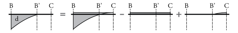
Lastly, to get to the maximum deflection point (point B'), we need to find the value of the partial parabola 'd'. This is more difficult than it looks, because recall that for the parabola areas shown in Figure 5.7, one end of the parabolic shape has to have a zero slope. This is not the case for area 'd'. Therefore, we need to consider the whole 'shear diagram' between points B and C as shown in Figure 5.13. The area 'd' may be calculated as the sum of three different areas. First, a parabola that goes all the way from B to C (with zero slope at point C) can be calculated easily as $LM/3$. Then subtract from that the area of the rectangle shown (of height $7.7/EI$). This means that we subtracted the area of the big parabola above the zero line and the area of the little parabola above the zero line. So we have to add that little parabola back in using $2LM/3$. The result of this is an area for 'd' of $-72/EI$, giving a total deflection at point B' of $-339/EI$. Since the deflection will move in the opposite direction to the right of point B', we know that this is the location of maximum deflection. To find it in $\mathrm{mm}$:
\begin{align*} \Delta_{B'} &= \frac{-339\mathrm{\,kNm^3}}{EI} \\ \Delta_{B'} &= \frac{-339\mathrm{\,kNm^3}}{200000\mathrm{\,MPa}(125.0\times 10^6\mathrm{\,mm^4})} \\ \Delta_{B'} &= \frac{-339\times 10^12\mathrm{\,Nmm^3}}{200000\mathrm{\,MPa}(125.0\times 10^6\mathrm{\,mm^4})} \\ \Delta_{B'} &= 13.6\mathrm{\,mm} = \Delta_{max} \end{align*}
The resulting deflection diagram ($\Delta$) in Figure 5.12 is composed entirely of cubic curves and shows the exact displaced shape of the beam. Notice the kink in the shape at point C (the location of the pin) where the slope changes abruptly as we would expect.