 Learn About Structures
Frame structures are more complex than beams because they do not necessarily all lie along a straight line as beams do. In frames, there can be both vertical members and members that are inclined on an angle. The first part of this section will discuss the types of loads on inclined members and how to deal with them. Then, it will explain the method that is used to analyse determinate frames (using the same methods that we used previously for determinate beams).
Inclined Loads
For members that are inclined on an angle, it is often most convenient to analyse them by first transforming all the loads on the member into the local member axis direction (perpendicular and parallel to the inclined member). This process is illustrated in Figure 4.7.
Sample geometry for an inclined member is shown at the top of Figure 4.7. Four different types of inclined loadings are shown in the figure.
The first type shows the transformation of point loads on an inclined member into parallel and perpendicular components.
The second type (`wind-type') is typical of distributed loadings caused by wind or other pressure-type loadings. The distributed load is applied directly perpendicular to the inclined member and is distributed along the diagonal length of the member ($L/cos\theta$ in this case). Since the load is already perpendicular to the member, no transformation is needed.
The third type ('dead-type') is a distributed load that is not applied perpendicular to the member. In this case, it is aligned with the global vertical axis direction to simulate the effect of a vertical gravity (or 'dead') load. This type of load is also distributed along the diagonal length of the member since the source of the load (in this case, the dead weight of the member) is also distributed along the diagonal length. In this case, a direct trigonometric transformation may be used to split the vertical distributed load into two different components, one perpendicular to the member (which will cause shear and bending) and one parallel to the member (which will cause axial load) as shown in the figure.
The fourth and final type (`snow-type') is a distributed load which is not perpendicular to the member and is also not distributed along the member length, but along the horizontal projection of the member (in this case, the distance $L$). For the case of a snow load, only a certain amount of snow can fall from a certain area of sky, so the greater the inclination of the member, the longer the length that the snow will be spread out over (making the load per unit of member length lower). The total vertical load here will be equal to $w_{snow}L$, which is less than the corresponding total vertical load from the dead load case, which was equal to $w_{dead}L/\cos\theta$. Before the snow-type distributed load can be split into perpendicular and parallel components, it must be spread evenly over the diagonal length of the member (instead of being spread evenly over the horizontal projection of the member). If we split the total vertical load $w_{snow}L$ over the total diagonal length $L/\cos\theta$ then we get a new vertical distributed load equal to $w_{snow}\cos\theta$ which is now distributed along the diagonal length of the member. From here, the load may be divided into perpendicular and parallel components as was done for the dead-type load, which results in the components shown in Figure 4.7.
Method for Analysing Determinate Frames
Analysing determinate frames is very similar to analysing determinate beams, except that you need to split up the frame into separate members so that they can each be analysed individually as beams. Frames also have the added complexity of potentially inclined members as well as the inclusion of axial forces in the analysis, which we previously neglected when we were analysing beams.
The general steps for analysing a determinate frame are:
- Use equilibrium to find all reaction forces.
- Split the frame into separate members.
Any point load or moment which acts directly on a joint between two or more members must be placed on only ONE of the members when they are split up. It does not matter which member gets the point load, as long as it is only on one.
- Find all of the forces at the ends of each member (at either member ends, or at cuts between that member and the adjacent member) using equilibrium on free body diagrams of each member on their own.
- Resolve all of the loads on the member (end loads and moments as well as loads along the length of the member) into the local member axis directions (i.e. perpendicular to and parallel to the member).
- Now the axial moment, shear force and bending moment diagrams may be found by solving each member as if it was a separate beam (see see Section 4.3).
- (As required) Use the results from each member to draw overall axial force, shear force and bending moment diagrams for the entire frame structure.
Example
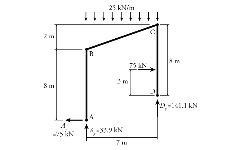
The analysis of determinate frames will be demonstrated using the example structure shown in Figure 4.8. Draw axial, shear and moment diagrams for all members of the structure.

As a first step, we can check that the structure is stable and determinate using the methods from Chapter 2. Using equation \eqref{eq:deg-indet}:
\begin{equation} \boxed{i_e = 3m + r - (3j + e_c) } \label{eq:deg-indet} \tag{1} \end{equation} \begin{align*} i_e &= 3m + r - (3j + e_c) \\ &= 3(3) + 3 - (3(4) + 0) \\ & = 0 \end{align*}
Since $i_e = 0$ then the structure is determinate. It is also stable since there are no collapse mechanisms present.
The next step in the analysis is to find the reaction forces. In this structure there are three reaction forces, $A_x$ and $A_y$ at the left pin, and $D_y$ at the right roller. We will find the reactions using equilibrium on the entire structure. The free body diagram of the structure is shown in Figure 4.9.
Starting with the moment equilibrium about point A to find the vertical reaction at D ($D_y$):
\begin{align*} \curvearrowleft \sum M_A &= 0 \\ -75(5)-25(7)(3.5)+D_y(7) &= 0 \\ D_y &= +141.1\mathrm{\,kN} \end{align*} \begin{equation*} \boxed{D_y = 141.1\mathrm{\,kN} \uparrow} \end{equation*}
For horizontal equilibrium, the horizontal reaction at A ($A_x$) is originally assumed to be positive (pointing to the right):
\begin{align*} \rightarrow \sum F_x &= 0 \\ A_x + 75 &= 0 \\ A_x &= -75\mathrm{\,kN} \end{align*}
But the negative solution tells us that $A_x$ actually points to the left (as shown in Figure 4.9):
\begin{equation*} \boxed{A_x = 75\mathrm{\,kN} \leftarrow} \end{equation*}
Vertical equilibrium:
\begin{align*} \uparrow \sum F_y &= 0 \\ A_y - 25(7) + D_y &= 0 \\ A_y - 25(7) + 141.1 &= 0 \\ A_y &= +33.9\mathrm{\,kN} \end{align*} \begin{equation*} \boxed{A_y = 33.9\mathrm{\,kN} \uparrow} \end{equation*}
Now, the structure must be divided into separate members. Our structure will be divided into three members, AB, BC, and CD. We will go through each in turn, solving for all the unknown end forces, axial force, shear force and moment before moving on to the next member. The free body diagram and solution for member AB is shown in Figure 4.10.
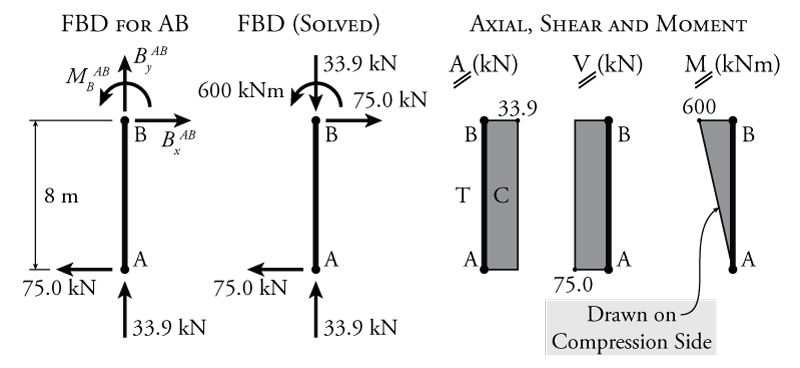
The free body diagram (FBD) on the left of Figure 4.10 shows all of the information that is currently known about member AB. It contains the known reactions at the base $A_x$ and $A_y$. In addition, the unknown forces at the cut at point B are also shown. To form the FBD for member AB, the structure had to be cut at point B. Since the structure is continuous at that point, we know that vertical and horizontal forces and a moment must be transmitted across the cut. Since we don't know anything about these forces yet, they are all drawn in the positive direction. The notation $B_x^{AB}$ means: "the force at point B in the x-direction, acting on member AB." Likewise, $M_B^{AB}$ means: "the moment at point B acting on member AB."
The FBD, has three unknowns: $B_x^{AB}$, $B_y^{AB}$, and $M_B^{AB}$. We can solve for these three unknowns using the equations of equilibrium:
\begin{align*} \curvearrowleft \sum M_B &= 0 \\ M_B^{AB} - 75(8) &= 0 \end{align*} \begin{equation*} \boxed{M_B^{AB} = 600\mathrm{\,kNm} \curvearrowleft} \end{equation*} \begin{align*} \rightarrow \sum F_x &= 0 \\ B_x^{AB} - 75 &= 0 \end{align*} \begin{equation*} \boxed{B_x^{AB} = 75.0\mathrm{\,kN} \rightarrow} \end{equation*} \begin{align*} \uparrow \sum F_y &= 0 \\ B_y^{AB} + 33.9 &= 0 \end{align*} \begin{equation*} \boxed{B_y^{AB} = 33.9\mathrm{\,kN} \downarrow} \end{equation*}
The resulting solved FBD is shown in Figure 4.10.
Now that we know all of the forces acting on member AB, we can use the methods of beam analysis to find the axial, shear and moment diagrams which are shown in Figure 4.10.
The construction of the axial force diagram is similar to the shear force diagram, starting at one end, forces that are parallel to the member that cause compression, move the axial force diagram one way, and forces that cause tension, move it the other way. It doesn't matter which way is which on the diagram, as long as the compression and tension sides of the diagram are indicated. The compression side of the axial force diagram is shown with a `C' in the figure. In this case, we can start at point A, assuming that the member is fixed at the other end (point B). The vertical reaction force at A of $49.5\mathrm{\,kN}$ causes the member to go in compression, so we move the axial force diagram to the right by the same amount and indicate that side as being in compression. There is no other load parallel to the member until point B, which has a force of $49.5\mathrm{\,kN}$ that would cause tension in the member if it pushes it away from B (assume that the force acts just below point B). This pushes the axial force diagram back to the left, meeting up with the member axis at 0.
The shear and moment diagrams for this member are simple and were constructed moving from bottom to top. The moment diagram is 'drawn on the compression side.' This means that for whichever side of of the member that shows a moment on the moment diagram, the extreme fibre on that side of the beam will be in compression. For this member AB, all of the moment is on the left side of the member. Therefore the left side of the member is in compression (and the right side is in tension).
Now that member AB has been completely solved, we can move on to the next member, member BC, which is shown in Figure 4.11.
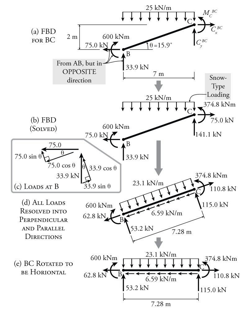
Part (a) of Figure 4.11 shows a free body diagram of member BC with all of the information that is currently known. Since members AB and BC are on either side of the cut at point B, the forces and moments must be transferred at that point. So, we can take the forces at point B from member AB and apply them to point B on member BC; however, we must be sure to reverse the direction of the forces, since forces and moments must be equal and opposite on either side of a cut (as previously discussed in Section 1.6). The horizontal force at the cut at B changes direction from right to left, the vertical force changes from down to up, and the moment changes from counter-clockwise to clockwise. Again, there are three unknown forces/moments at point C due to the cut between member BC and member CD: $C_x^{BC}$, $C_y^{BC}$, and $M_C^{BC}$. These may be found using equilibrium:
\begin{align*} \curvearrowleft \sum M_C &= 0 \\ M_C^{BC} + 25(7)(3.5) - 33.9 (7) - 75.0 (2) - 600 &= 0 \end{align*} \begin{equation*} \boxed{M_C^{BC} = 374.8\mathrm{\,kNm} \curvearrowleft} \end{equation*} \begin{align*} \rightarrow \sum F_x &= 0 \\ -75 + C_x^{BC} &= 0 \end{align*} \begin{equation*} \boxed{C_x^{BC} = 75.0\mathrm{\,kN} \rightarrow} \end{equation*} \begin{align*} \uparrow \sum F_y &= 0 \\ 33.9 - 25(7) + C_y^{BC} &= 0 \end{align*} \begin{equation*} \boxed{C_y^{BC} = 141.1\mathrm{\,kN} \uparrow} \end{equation*}
The resulting solved free body diagram is shown in Part (b) of Figure 4.11. Since member BC is an inclined member, we need to resolve all of the forces into the local member directions (i.e. perpendicular and parallel to the member) before we can find the axial, shear and moment on the member. This process is shown in Parts (c) and (d) of the figure. Part (c) shows how to convert the horizontal and vertical forces at point B into forces that are perpendicular and parallel to member BC. To do this, each force must be split into two components, one perpendicular and one parallel to member BC. The perpendicular components from each are then added together to get the total perpendicular point load at B:
\begin{align*} P_{perp} &= 75.0 \sin \theta + 33.9 \cos \theta \\ P_{perp} &= 75.0 \sin {15.9^\circ} + 33.9 \cos {15.9^\circ} \\ P_{perp} &= 53.2\mathrm{\,kN} \nwarrow \text{ (perpendicular to BC)} \end{align*}
and the parallel forces are summed to get:
\begin{align*} P_{para} &= -75.0 \cos {15.9^\circ} + 33.9 \sin {15.9^\circ} \\ P_{para} &= 62.8\mathrm{\,kN} \swarrow \text{ (parallel. to BC)} \end{align*}
The same process is followed for the point loads at point C.
Part (d) of Figure 4.11 shows the resulting point loads (parallel and perpendicular) at either end of the member. It also shows the distributed load resolved into the local axis (member) directions. The snow-type distributed load on the beam is resolved into the perpendicular and parallel directions using the expressions previously shown in Figure 4.7:
\begin{align*} w_{perp} &= w_{snow} \cos^2 \theta \\ w_{perp} &= 25 \cos^2 {15.9^\circ} \\ w_{perp} &= 23.1\mathrm{\,kN/m} \searrow \\ w_{para} &= w_{snow} \cos \theta \sin \theta \\ w_{para} &= 25 \cos {15.9^\circ} \, \sin {15.9^\circ} \\ w_{para} &= 6.59\mathrm{\,kN/m} \swarrow \end{align*}
The moments are not affected when translating the forces into the perpendicular and parallel directions.
Part (e) of Figure 4.11 shows the same fully solved free-body diagram as Part (d) but simply rotated to be horizontal so that it is easier to analyse. Note also that the length of the member itself ($\sqrt{7^2 + 2^2} = 7.28\mathrm{\,m}$) is longer than the horizontal projection ($7\mathrm{\,m}$).
Now that all of the loads on member BC are known, the axial, shear and moment diagrams may be constructed using the methods for beam analysis. This process is shown in Figure 4.12.

The axial force diagram is not constant for member BC, as shown in Figure 4.12, because the snow-type distributed load on the member has a parallel component which acts along the length of the member. This parallel distributed load may be called a traction along the length of the member. Moving from left to right, the member starts with a tension of $62.8\mathrm{\,kN}$ which is then steadily increased by a traction in the same direction of $6.59\mathrm{\,kN/m}$, which moves the axial force diagram further towards the tension side. This results in a slope on the axial force diagram also equal to $6.59\mathrm{\,kN/m}$. At the right end of the member, a final compression (in the opposite direction) of $110.8\mathrm{\,kN}$ brings the axial force diagram back to zero.
The shear force and bending moment diagrams are constructed as before, with particular attention to the slope of the moment diagram at any point being directly equal to the value of the shear force diagram at the same point. The moment diagram shown in Figure 4.12, starts with a jump up due to the clockwise moment at point B, then moves even higher due to the shear between points B and B', before dropping once again between points B' and C. It is important to identify the maximum moment and where that maximum moment occurs. The value of the maximum moment is easily found by adding the moment at point B ($600\mathrm{\,kNm}$) to the area under the shear force diagram between points B and B' (a triangle with a height of $53.2\mathrm{\,kN}$). To find the area of that triangle, we need to know the length of the base. This may be found using similar triangles as shown (the total length of the member multiplied by the height of the small triangle divided by the total height of both triangles). In this case, the length of the smaller triangle is $2.303\mathrm{\,m}$ as shown. This is the location of the point of maximum moment, which should be identified on the moment diagram. Using this length, the area under the shear force diagram between points B and B' is equal to $0.5(53.2)(2.303)=61.2\mathrm{\,kNm}$. This gives a maximum moment of $600 + 61.2 = 661.2\mathrm{\,kNm}$ at a location $2.303\mathrm{\,m}$ from point B (as shown in shown in Figure 4.12).
Since the shape of the shear force diagram is linear, then the shape of the moment diagram should be parabolic. The shape of the parabola can be easily determined by sketching in the slope of the moment diagram at both ends as shown in Figure 4.12 and by identifying locations of zero slope, which are the points where the shear force diagram equals zero. This moment diagram is again drawn on the compression side of the member and it can be seen that, as mentioned previously, the point moments at the ends of the member point towards the compression side of the beam at either end.
Now that member BC is completely solved, we can move onto the final member, member CD, which is shown in Figure 4.13.
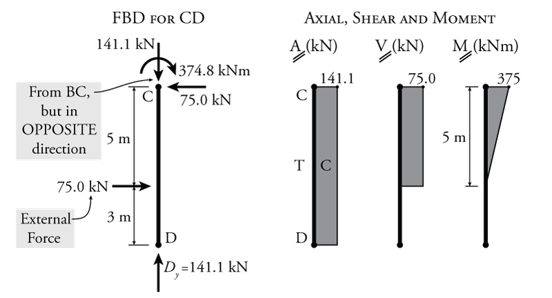
The free body diagram of member CD shown in Figure 4.13 includes all of the information that is known up to this point (including the opposite direction forces from member BC on the other side of the cut at point C). As this figure shows, there are no unknown forces that need to be found for member CD. This is typically the case with the final member in a frame analysis. We have already determined the forces at point D when we found the reactions using global equilibrium; however, we can use equilibrium on member CD as a check that we have solved the rest of the frame properly. If we do this check and equilibrium is not satisfied, then we have made a mistake in one of the previous steps. So, let's check equilibrium for member CD:
\begin{align*} \curvearrowleft \sum M_C &= 0 \\ -374.8 + 75(5) &= 0 \; \checkmark \end{align*} \begin{align*} \rightarrow \sum F_x &= 0 \\ 75 - 75 &= 0 \; \checkmark \end{align*} \begin{align*} \uparrow \sum F_y &= 0 \\ 141.1 - 141.1 &= 0 \; \checkmark \end{align*}
All of the equilibrium equations are satisfied, so we can have some confidence that our solution is correct.
Knowing all of the forces on member CD, we can construct the axial, shear and moment diagrams using beam analysis methods as shown in Figure 4.13 (try it yourself!).
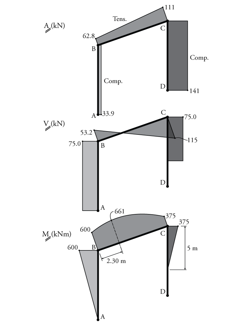
Now that all of the axial, shear and moment diagrams have been constructed for each member, the last optional step is to combine them onto a single diagram which shows the axial, shear and moment for the entire structure. These summary diagrams are shown in Figure 4.14.