 Learn About Structures
What is static equilibrium?
Technically, a body (or structure) is in static equilibrium if it is not accelerating. This means that it is moving at a constant velocity. Why is this the case? According to relativity (Einstein), it is not possible to tell if an object is moving or not from the point of view of an observer on the object if that object is moving at a constant velocity. If you are sitting in a train, moving at constant velocity, it feels just like you are sitting still (except for any bumps in the road that momentarily change your velocity). You can comfortably enjoy a nice cup of hot coffee without spilling it all over yourself (again, unless you hit a bump). You, and the coffee, are in static equilibrium.
If you hit a bump, your velocity changes. You may start moving vertically a bit upwards after hitting the bump and then downwards again due to gravity. A change in velocity is always caused by an acceleration. Inside the train, you can tell that your velocity has changed because you can feel the acceleration manifested as an unbalanced force on your body. This is because acceleration is, in turn, always associated with some unbalanced (net) force on a body. Another example of this is the experience of a passenger in an accelerating car. As the car accelerates forward, you would feel a force pushing you back into your seat. Once the car stops accelerating and maintains a constant velocity, that force goes away.
The relationship between acceleration and the force caused by that acceleration is given by Newton's second law:
\begin{equation} \tag{1} F=ma \end{equation}
where $F$ is the net unbalanced force on an object, $m$ is the mass of the object, and $a$ is the acceleration applied to that object.
As civil engineers, we are used to seeing this relationship in terms of the force and acceleration caused by gravity. Gravity causes a constant acceleration towards the centre of the earth with a magnitude of $g=9.81\mathrm{\,m/s^2}$. Applying Newton's second law, and using $g$ as the acceleration, we get:
\begin{equation} \tag{2} F_g=mg \end{equation}
where $F_g$ is the force due to gravity and $g$ is the acceleration due to gravity. This force is constantly being applied to all objects on earth (in proportion to their mass). When we are stationary on the surface of the earth, that is because this force is being balanced by a constant reaction force from the ground that is keeping us in place. If we are sitting, we feel a constant force of the seat against our bottoms. If we are standing, we feel it against our feet. The force never goes away. These forces counterbalance the force of gravity causing us to remain in static equilibrium and stopping us from accelerating. Remove someone's chair and the reaction force is removed. This results in a loss of static equilibrium, and an unbalanced force (the force of gravity) which causes an acceleration towards the ground and a sore bottom (at which point the person hits the ground and equilibrium is achieved once more). You can imagine that if we build a structure, we want to ensure that that structure stays in static equilibrium. If a structure is not in equilibrium, that means it is accelerating, which is rarely a good situation. Accelerations on structures are encountered in the design of structures for dynamic loadings such as wind or earthquake loads; however, such situations are beyond the scope of this book.
How Can You Tell When a Structure is in Equilibrium?
A structure is in static equilibrium when there is no net force or moment on it. If a structure that is initially stationary has a net force, it will start to move and will no longer be in equilibrium. If a structure that is initially stationary has a net moment (or torque), then it will start to rotate. To avoid these situations, all of the forces in every direction must counterbalance each other. The same thing goes for the moments. This can be evaluated by adding up the components of the forces in each orthogonal ordinate direction ($x$, $y$, and $z$) and making sure that the sum of the forces in each direction add up to zero:
\begin{equation} \label{eq:Equil3D1} \tag{3} \sum_{i=1}^{n}{F_{xi}} = 0; \sum_{i=1}^{p}{F_{yi}} = 0; \sum_{i=1}^{q}{F_{zi}} = 0 \end{equation}
where $F_{xi}$, $F_{yi}$, and $F_{zi}$ are the individual force components in the $x$-, $y$- and $z$- directions, respectively (out of $n$, $p$, and $q$ total force components in the same directions). In 2D problems, only the $x$ and $y$ directions would be considered. Similarly, for the moments, the sum of the moments around each ordinal axis may be summed to make sure that the sums equal zero:
\begin{equation} \label{eq:Equil3D2} \tag{4} \sum_{i=1}^{n}{M_{xi}} = 0; \sum_{i=1}^{p}{M_{yi}} = 0; \sum_{i=1}^{q}{M_{zi}} = 0 \end{equation}
In 2D problems, there is only one rotational axis (the $z$-axis), and so only $M_z$ would be considered. If all of these equilibrium equations are satisfied (if they all sum to zero), then the system is in static equilibrium. If they are not, then the system is accelerating! Hence, in 2D, there are three applicable equations of equilibrium:
\begin{equation}\label{eq:Equil2D}\tag{5} \boxed{ \sum_{i=1}^{n}{F_{xi}} = 0; \sum_{i=1}^{p}{F_{yi}} = 0; \sum_{i=1}^{q}{M_{zi}} = 0 } \end{equation}
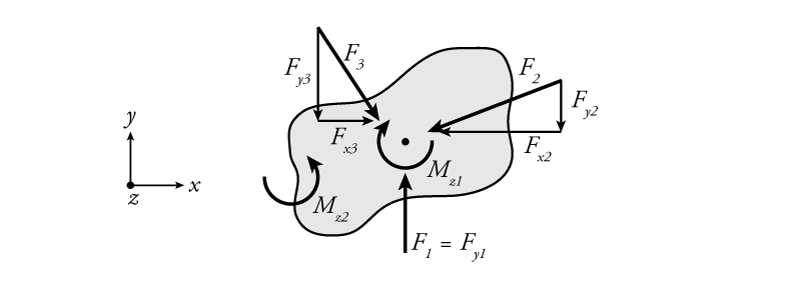
An example of 2D equilibrium on a generic rigid body is shown in Figure 1.1. This figure is a free body diagram (or FBD), meaning that it shows the full system without any external connections and it includes all of the forces that are acting on the system. In the figure, the $x$-axis is horizontal, the $y$ axis is vertical, and the $z$-axis is out of the plane of the page. The $z$-axis is included (even though this is a 2D example) because rotations and moments in the $xy$ plane occur around the $z$-axis. If this system is not accelerating (i.e. it is in static equilibrium, then the equilibrium equations in \eqref{eq:Equil2D} apply as follows:
\begin{align} \tag{6} \sum_{i=1}^{n}{F_{xi}} = 0 \\ F_{x3} - F_{x2} = 0 \\ \sum_{i=1}^{p}{F_{yi}} = 0 \\ F_{y1} - F_{y2} - F_{y3} = 0 \\ \sum_{i=1}^{q}{M_{zi}} = 0 \\ M_{z2} - M_{z1} = 0 \end{align}
In this example, all of the forces ($F_1$, $F_2$, and $F_3$) are applied directly through a single point (they are coincident), so they do not create any moment on the rigid body. The only moments on the body are the point moments $M_{z1}$ and $M_{z2}$ and for the body to be in equilibrium, these two moments must have equal magnitude and act in the opposite rotational direction.
If all of the forces are not coincident through the same point, then they also cause moments and must be considered in the moment equilibrium equation. To find the moment caused by a force on a rigid body, you need to define a reference point on the body. Any reference point is okay (any point on the body), as long as the same reference point is used to calculate all of the moments. To calculate the moment caused by a force, the force is multiplied by the moment arm or eccentricity which is equal to the perpendicular distance between the force and the reference point. That is, it is the distance between the force vector (the arrow) and a line that is parallel to the force vector and also runs through the reference point. It is also important to consider the direction of the moment caused by the force relative to the reference point. Generally, one rotation direction is considered positive and the other is considered negative. In this text, counter clock-wise (CCW~$\curvearrowleft$) rotations will be considered positive and clock-wise rotations (CW~$\curvearrowright$) will be considered negative.
This calculation of the moments for two different reference point locations is illustrated by Figure 1.2. In the figure, the perpendicular distance for each force is shown as $e_i$ ($e$ for 'eccentricity'). For the reference point location on the left-side rigid body in the figure, the moment equilibrium equation is:
\begin{align} \tag{7} \sum_{i=1}^{q}{M_{zi}} = 0 \\ M_{z2} - M_{z1} + F_2 e_2 + F_1 e_1= 0 \end{align}
The moments $M_{z2}$, $F_1 e_1$ and $F_2 e_2$ are all positive because they both would all cause a counter clock-wise (CCW~$\curvearrowleft$) rotation of the rigid body around the reference point (if it was not in equilibrium). Likewise, $M_{z1}$ is negative because it would cause a clock-wise (CW $\curvearrowright$) rotation. The horizontal force $F_3$ does not produce any moment for this equilibrium equation because it is concurrent with the reference point (it passes through that point).
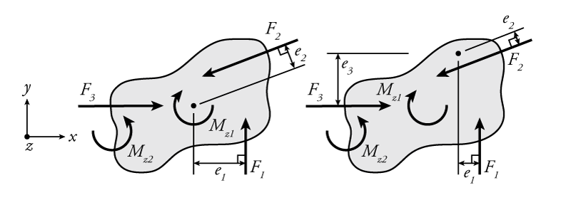
For the reference point location on the right-side rigid body in the figure, the moment equilibrium equation is:
\begin{equation} \tag{8} M_{z2} - M_{z1} - F_2 e_2 + F_1 e_1 + F_3 e_3 = 0 \end{equation}
Notice that since the reference point location has changed, the sign of $F_2 e_2$ has changed from $+$ to $-$ because the moment $F_2 e_2$ would now cause a clock-wise (CW $\curvearrowright$) rotation around the reference point. Of course, the magnitudes of the moment arms $e_1$ and $e_2$ have also changed. In addition, there is an additional term in the moment equilibrium because $F_3$ is no longer concurrent with the reference point and so, therefore, produces a positive (CCW $\curvearrowleft$) moment of $F_3 e_3$. This shows that it may be convenient to choose a reference point that is concurrent with one or more of the forces because it reduces the number of terms in the moment equilibrium equation. This may make a problem easier to solve. The point moments $M_{z1}$ and $M_{z2}$ have not changed. They are not dependent on the location of the reference point and are always simply added or subtracted from the moment equilibrium depending on their rotational direction.
Whether you use the reference point location shown on the left or right side of the Figure 1.2, the equilibrium will not change. If the body is in equilibrium, then the moments will all add up to zero regardless of the location of the reference point that you choose.
Solving for Unknown Forces and/or Moments using Equilibrium
Knowing the equations of static equilibrium \eqref{eq:Equil3D1} and \eqref{eq:Equil3D2}, if all the forces are known it is a simple matter to check and see if a body is in equilibrium or not by simply applying those equations and seeing if they are satisfied (i.e. the forces and moments add up to zero in each direction). This ability, in itself, is not terribly useful for structural analysis. Unless we are studying a system that is subject to dynamic wind or earthquake loading, then we already know that our structures are in equilibrium since they are fixed to the ground. A much more common problem in structural analysis is that we know some of the forces acting on a structure but not all of them. If this is the case, then we can use the fact that we know that a structure is in equilibrium to turn the problem around. If we take it as a given that the equilibrium equations are satisfied, then we can use the equations to solve for up to six unknown forces or moments on the structure in 3D or up to three unknown forces or moments in 2D. In 2D (equation \eqref{eq:Equil2D}), since we have three independent equilibrium equations, then we can solve for three unknown forces or moments using algebra. The equations are called independent because each equation provides unique information about the system.
Example
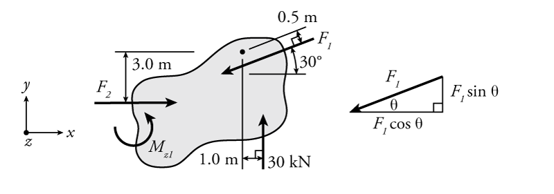
For example, Figure 1.3 shows a rigid body with only one known force (30 kN vertical), two unknown forces ($F_1$ and $F_2$), and one unknown moment ($M_{z1}$), giving three total unknowns.
If we can assume that the object is in equilibrium, then we can solve for the unknown forces and moment using our three equilibrium equations for 2D systems from equation \eqref{eq:Equil2D}. This is equivalent to finding the forces and moment that would be necessary for the body to be in equilibrium.
First, using vertical equilibrium:
\begin{align*} \sum_{i=1}^{p}{F_{yi}} &= 0\\ 30 - F_1 \sin{30 ^\circ} &= 0\\ F_1 &= \dfrac{30}{\sin{30^\circ}}\\ F_1 &= 60 \mathrm{\,kN}\swarrow \end{align*}
where up is considered to be the positive direction. Since the result is positive, the direction of the arrow for $F_1$ in Figure 1.3 was correct (down and to the left). If this value came out negative, then we would know that the arrow should actually be drawn in the opposite direction (up and to the right). Then, using horizontal equilibrium:
\begin{align*} \sum_{i=1}^{n}{F_{xi}} &= 0\\ F_2 - F_1 \cos{30^\circ } &= 0\\ F_2 &= (60\mathrm{\,kN}) {\cos{30^\circ}}\\ F_2 &= 52\mathrm{\,kN}\rightarrow \end{align*}
where right is considered to be the positive direction. Again, since the result is positive, then it was correct to draw $F_2$ pointing towards the right. Last, the moment equilibrium:
\begin{align*} \sum_{i=1}^{q}{M_{zi}} &= 0 \\ M_{z1} - F_1 (0.5\mathrm{\,m}) + F_2 (3.0\mathrm{\,m}) + 30\mathrm{\,kN} (1.0\mathrm{\,m}) &= 0\\ M_{z1} - 60\mathrm{\,kN} (0.5\mathrm{\,m}) + 52\mathrm{\,kN} (3.0\mathrm{\,m}) + 30\mathrm{\,kN}(1.0\mathrm{\,m}) &= 0\\ M_{z1} &= -156\mathrm{\,kN}\\ M_{z1} &= 156\mathrm{\,kN}\curvearrowright \end{align*}
where counter clock-wise (CCW $\curvearrowleft$) rotations are considered to be positive. Since the resulting value for $M_{z1}$ is negative, this means that the moment arrow was assumed to be in the wrong direction in Figure 1.3 and the moment $M_{z1}$ required for equilibrium must be in the clock-wise (CW $\curvearrowright$) direction.