 Learn About Structures
The slope-deflection method relies on the use of the slope-deflection equation, which relate the rotation of an element (both rotation of the nodes at the ends of the element and rigid body rotation of the entire element) to the total moments at either end. The ultimate goal of the slope deflection equations is to find the end moments for each member in the structure as a function of all of the DOFs associated with the member. From there, we can apply equilibrium conditions at all of the joints to solve for the unknown rotations. This is the system of equations that we will have to solve: the equations are the equilibrium equations for each node and the unknowns are the translations and rotations of the nodes.
The first step is that we need an expression for the moment at each end of an arbitrary member in an indeterminate structure in terms of the rotations and translations of the nodes at either end. If there are loads between the nodes (i.e. distributed loads, point loads, or moments along the length of the member), then we will need a way to consider the effect of those as well.
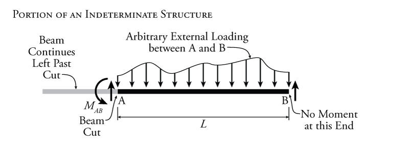
Such an arbitrary member that we will use to develop the slope deflection equations is shown in Figure 9.2. We will consider that this member is a smaller part of a larger structure, so at each end there is a section cut, and at each cut there is a shear force and a moment. We will be most concerned about the moments at the ends. At the left end, the moment is labelled $M_{AB}$, where the first letter in the subscript is the node that the moment is applied to (in this case node A) and the second letter is the node at the other end of the member (in this case node B). At the right end, the moment at the cut is labelled $M_{BA}$ since the moment is applied at node B, and the other end of the member is at point A. This naming convention allows us to distinguish between the moments at either end of a member (e.g. $M_{AB}$ and $M_{BA}$) and between moments from different members that all must be in equilibrium at a single node (e.g. $M_{AB}$ is the moment applied to node A by member AB and $M_{AC}$ would be the moment applied to node A by member AC).
The member shown at the top of Figure 9.2 may also have some arbitrary external loading between the two end nodes as shown.
It is important to point out that, as shown in Figure 9.2, since the slope-deflection method will involve evaluating equilibrium of individual point moments at different nodes, then we are most interested in the absolute rotational direction of the moments, not the internal moment sign convention (see previous Section 1.6). So, in these analyses we will consider all counter-clockwise moments to be positive and all clockwise moments to be negative.
Based on the positive point moment sign convention (counter-clockwise), the general deformed shape of member is shown at the bottom of Figure 9.2. Each end of the element (at node A or B) has its own rotation relative to the element's initial position ($\theta_A$ and $\theta_B$) as shown in the figure. In addition, node B can translate vertically by an amount $\Delta$ relative to node A as also shown. This will result in a rotation of the entire element. We can represent this overall rigid body rotation by the rotation of the element chord (i.e. a straight line connecting point A and B). The rotation of this chord (with the greek symbol psi $\psi$) is equal to:
\begin{equation} \boxed{ \psi = \frac{\Delta}{L} } \label{eq:chord-rotation} \tag{1} \end{equation}
where $\Delta$ is the vertical translation of node B relative to node A, and $L$ is the total length of the element between nodes A and B. Note that we are assuming that the rotations are small. There is no relative horizontal translation between nodes A and B since we are assuming that our elements are axially rigid for the slope-deflection method.
Due to the chord rotation $\psi$, not all of the rotation at each end ($\theta_A$ and $\theta_B$) will cause internal moment in the member. It is only the amount of rotation relative to the chord of the member that will cause internal moment. If we would like to find only the rotation at each end that is associated with the internal moment in the element, then we must remove the component of the total rotation that is caused by the chord rotation, as shown in the lower diagram in Figure 9.2. The relative rotations between the beam end and the chord are then equal to:
\begin{align} \theta_{A,rel} &= \theta_A - \psi \label{eq:slope-def-rel-rotA} \tag{2} \\ \theta_{A,rel} &= \theta_A - \frac{\Delta}{L} \label{eq:slope-def-rel-rotB} \tag{3} \\ \theta_{B,rel} &= \theta_B - \psi \label{eq:slope-def-rel-rotC} \tag{4} \\ \theta_{B,rel} &= \theta_B - \frac{\Delta}{L} \label{eq:slope-def-rel-rotD} \tag{5} \end{align}
Continuing to try and find an expression for the moment at each end of the element in terms of the DOF translations and rotations, we can take advantage of superposition to determine the total internal moments caused by both the end moments and by the loads in between the element end nodes. The three components of that superposition are shown in Figure 9.3. The internal moment due to the end moments $M_{AB}$ and $M_{BA}$ are easy to construct. The internal moment due to the external loading between A and B is more difficult to handle because it changes for different types of loading. So, at this stage, we will consider that moment diagram caused by the external loading between A and B to have an arbitrary shape as shown in the figure.

This has all given us a relationship between the end moments and external forces to the internal moments. If we can now relate these internal moments to the rotation and translation at both ends of the beam, then we will, in turn, be able to relate the nodal rotations and translations to the end moments and external forces. We can use the moment area method from Chapter 5 to find the rotations and translations caused by the internal moments (converted to curvatures of course) as shown in Figure 9.4. Each superimposed moment diagram cause a different rotation at either end of the member. We will be able to use superposition to add the effects of all three. Of course, the rotations that we are talking about here are the relative rotations at the ends of the element $\theta_{A,rel}$ and $\theta_{B,rel}$ (which are relative to the chord rotation); however, these are related to the total rotations $\theta_A$ and $\theta_B$ as described by equations \eqref{eq:slope-def-rel-rotA} to \eqref{eq:slope-def-rel-rotD}. So, there will be three different relative rotations at each end that will all sum up to the total relative rotation at each end based on superposition:
\begin{align} \theta_{A,rel} &= \theta_{A,rel1} + \theta_{A,rel2} + \theta_{A,rel3} \label{eq:rel-rot-totalA} \tag{6} \\ \theta_{B,rel} &= \theta_{B,rel1} + \theta_{B,rel2} + \theta_{B,rel3} \label{eq:rel-rot-totalB} \tag{7} \end{align}
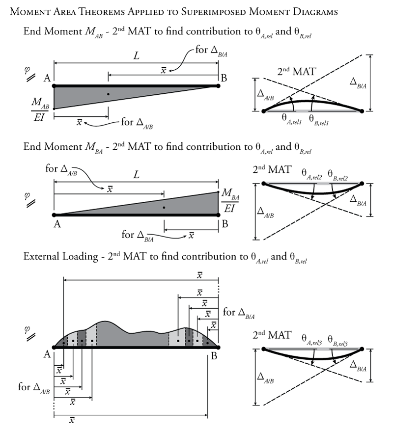
To determine each relative rotation component using the moment area theorem, all of the required curvature diagrams are shown in Figure 9.4 along with the appropriate application of the second moment area theorem for each on the right side of the figure. For the curvature caused by end moment $M_{AB}$:
\begin{align} \Delta_{A/B} &= \left( \frac{1}{2} \right) (L) \left( \frac{M_{AB}}{EI} \right) \left( \frac{L}{3} \right) = \frac{M_{AB}L^2}{6EI} \tag{8} \\ \Delta_{B/A} &= \left( \frac{1}{2} \right) (L) \left( \frac{M_{AB}}{EI} \right) \left( \frac{2L}{3} \right) = \frac{M_{AB}L^2}{3EI} \tag{9} \end{align}
and, since $\theta = \frac{\Delta}{L}$:
\begin{align} \theta_{A,rel1} &= \frac{\Delta_{B/A}}{L} = \frac{M_{AB}L}{3EI} \tag{10} \\ \theta_{B,rel1} &= -\frac{\Delta_{A/B}}{L} = -\frac{M_{AB}L}{6EI} \tag{11} \end{align}
As Figure 9.4 shows, $\theta_{A,rel1}$ should be positive and $\theta_{B,rel1}$ should be negative.
Similarly, for the curvature caused by end moment $M_{AB}$ as shown in Figure 9.4:
\begin{align} \theta_{A,rel2} &= -\frac{\Delta_{B/A}}{L} = -\frac{M_{BA}L}{6EI} \tag{12} \\ \theta_{B,rel2} &= \frac{\Delta_{A/B}}{L} = +\frac{M_{BA}L}{3EI} \tag{13} \end{align}
The last curvature diagram, the one based on the external loading between the end nodes A and B, is not precisely defined in Figure 9.4 because it depends on the loading. So, we will assume for now that we can find the moment of the area for use with the second moment area theorem and that we can use that to find $\theta_{A,rel3}$ and $\theta_{B,rel3}$:
\begin{align} \theta_{A,rel3} &= -\frac{\Delta_{B/A,ext}}{L} \tag{14} \\ \theta_{B,rel3} &= \frac{\Delta_{A/B,ext}}{L} \tag{15} \end{align}
Now we can find the total relative rotation at both nodes using equations \eqref{eq:rel-rot-totalA} and \eqref{eq:rel-rot-totalB}:
\begin{align} \theta_{A,rel} &= \frac{M_{AB}L}{3EI} - \frac{M_{BA}L}{6EI} -\frac{\Delta_{B/A,ext}}{L} \tag{16} \\ \theta_{B,rel} &= -\frac{M_{AB}L}{6EI} + \frac{M_{BA}L}{3EI} + \frac{\Delta_{A/B,ext}}{L} \tag{17} \end{align}
Substituting in equations \eqref{eq:slope-def-rel-rotA} and \eqref{eq:slope-def-rel-rotC}:
\begin{align} \theta_A - \psi &= \frac{M_{AB}L}{3EI} - \frac{M_{BA}L}{6EI} -\frac{\Delta_{B/A,ext}}{L} \label{eq:rot-in-terms-momA} \tag{18} \\ \theta_B - \psi &= -\frac{M_{AB}L}{6EI} + \frac{M_{BA}L}{3EI} + \frac{\Delta_{A/B,ext}}{L} \label{eq:rot-in-terms-momB} \tag{19} \end{align}
This gives us two expressions for the rotations of nodes A and B in terms of the end moment and the external force (assuming we can find $\Delta_{A/B,ext}$ and $\Delta_{B/A,ext}$ somehow using the second moment area theorem). The nodal translations are embedded in the parameter $\psi$ which is a function of the relative translation of the two end nodes as previously discussed.
What we want, though, is the reverse. We want expressions for the end moments $M_{AB}$ and $M_{BA}$ in terms of the nodal translations and rotations. To get these, all we have to do is rearrange the two simultaneous equations \eqref{eq:rot-in-terms-momA} and \eqref{eq:rot-in-terms-momB} to solve in terms of the end moments:
\begin{align} M_{AB} &= \frac{2EI}{L} (2 \theta_A + \theta_B - 3 \psi ) + \frac{2EI}{L^2} ( 2 \Delta_{A/B,ext} - \Delta_{B/A,ext} ) \label{eq:SD-IntA1} \tag{20} \\ M_{BA} &= \frac{2EI}{L} (\theta_A + 2 \theta_B - 3 \psi ) + \frac{2EI}{L^2} ( \Delta_{A/B,ext} - 2 \Delta_{B/A,ext} ) \label{eq:SD-IntA2} \tag{21} \end{align}
The second term in each of these equations (the one with $\Delta_{A/B,ext}$ and $\Delta_{A/B,ext}$) is caused by the external loading on the element between the two end nodes. We had speculated previously that it would be possible to find these second moment area theorem terms if we knew the loading, but there is an easier way.
Let's see what happens if we isolate the second terms of equations \eqref{eq:SD-IntA1} and \eqref{eq:SD-IntA2}. We can do this by looking at the case where all rotations and translations are equal to zero (i.e. $\theta=0$ and $\psi = 0$). If we do this, we get the following equations for $M_{AB}$ and $M_{BA}$:
\begin{align} M_{AB} &= \frac{2EI}{L^2} ( 2 \Delta_{A/B,ext} - \Delta_{B/A,ext} ) \label{eq:SD-IntB1} \tag{22} \\ M_{BA} &= \frac{2EI}{L^2} ( \Delta_{A/B,ext} - 2 \Delta_{B/A,ext} ) \label{eq:SD-IntB2} \tag{23} \end{align}
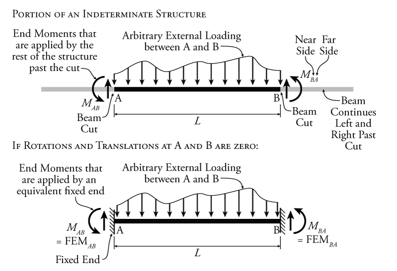
This does not help us on its own, but let's look at what is happening in the element when we set the rotations and translations to zero. This condition is illustrated in Figure 9.5. If we have zero rotation and zero translation at both ends of the element, it is as if the ends of the element have fixed supports at either end, as shown in the figure. This results in a ${3^\circ}$ indeterminate beam structure. But, if we can find the reaction moments at the fixed ends, those are the solution to $M_{AB}$ and $M_{BA}$ when $\theta=0$ at both ends and $\psi = 0$. Let's assume that we can easily solve for those reaction moments and call them $\text{FEM}_{AB}$ for the reaction support moment of the fixed end beam on the left side (equivalent to $M_{AB}$) and $\text{FEM}_{BA}$ for the reaction support moment of the fixed end beam on the right side (equivalent to $M_{BA}$).
Putting these fixed end moments back into equations \eqref{eq:SD-IntB1} and \eqref{eq:SD-IntB2}, we get:
\begin{align} \text{FEM}_{AB} &= \frac{2EI}{L^2} ( 2 \Delta_{A/B,ext} - \Delta_{B/A,ext} ) \label{eq:SD-IntC1} \tag{24} \\ \text{FEM}_{BA} &= \frac{2EI}{L^2} ( \Delta_{A/B,ext} - 2 \Delta_{B/A,ext} ) \label{eq:SD-IntC2} \tag{25} \end{align}
So, the second terms of equations \eqref{eq:SD-IntA1} and \eqref{eq:SD-IntA2} may be replaced by the fixed end moments. The resulting equations are called the slope-deflection equations:
\begin{equation} \boxed{ M_{AB} = \frac{2EI}{L} (2 \theta_A + \theta_B - 3 \psi ) + \text{FEM}_{AB} } \label{eq:SD-AB} \tag{26} \end{equation} \begin{equation} \boxed{ M_{BA} = \frac{2EI}{L} (\theta_A + 2 \theta_B - 3 \psi ) + \text{FEM}_{BA} } \label{eq:SD-BA} \tag{27} \end{equation}
where $M_{AB}$ is the end moment of element AB at node A, $M_{BA}$ is the end moment of element AB at node B, $\theta_A$ is the rotation of node A, $\theta_B$ is the rotation of node B, $\psi$ is the chord rotation as per equation \eqref{eq:chord-rotation}, $E$ is the material Young's modulus, $I$ is the element moment of inertia, and $L$ is the length of the element.
But how do we find the fixed end moment $\text{FEM}_{AB}$ and $\text{FEM}_{BA}$? Typically, the easiest way to evaluate these is to use a pre-calculated table such as the one shown in Figure 9.6. Using this table, the fixed end moments may be determined for different loading conditions. If there are multiple different loading conditions on the same elements (e.g. a distributed load and a point load), then the fixed end moments caused by those separate loading conditions may be simply added together using superposition to find the total $\text{FEM}_{AB}$ or $\text{FEM}_{BA}$ (separately at each end). When using this table, do not forget that counter-clockwise moments are positive and clockwise moments are negative. So, using Figure 9.6, for the point load diagram shown at the top left of the figure, the fixed end moment at the left end of the element would be $+\frac{PL}{8}$ and the fixed end moment at the right would be $-\frac{PL}{8}$.

The slope deflection equations from equations \eqref{eq:SD-AB} and \eqref{eq:SD-BA} may also be restated in a single equation as:
\begin{equation} \boxed{ M_{nf} = \frac{2EI}{L} (2 \theta_n + \theta_f - 3 \psi ) + \text{FEM}_{nf} } \label{eq:SD-NF} \tag{28} \end{equation}
where instead of referring to nodes A and B, it refers to node $n$, which is the near end (the end that you are finding the end moment for) and node $f$ is the far end (the node at the opposite end of the element).
If we have an element in the structure that has zero moment at one end then the entire analysis above may be redone to take advantage of the extra information. This can happen if the member has one end on an external pin or roller, it is the only member connected at that point, and it does not have any external point moment at that point. This situation is illustrated in Figure 9.7. For this situation, the analysis will result in the following modified slope-deflection equations:
\begin{equation} \boxed{ M_{rh} = \frac{3EI}{L} (\theta_r - \psi ) + \left( \text{FEM}_{rh} - \frac{\text{FEM}_{hr}}{2} \right) } \label{eq:SD-RH} \tag{29} \end{equation} \begin{equation} \boxed{ M_{hr} = 0 } \label{eq:SD-HR} \tag{30} \end{equation}
where node $r$ is the node at the rigid end (a continuous end or an end that has a fixed end support) and node $h$ is the node at the hinged or pinned end that cannot resist moment. Notice that, unlike equation \eqref{eq:SD-NF}, which has two different rotations $\theta_n$ and $\theta_f$, this equation only has one rotation $\theta_{r}$. This effectively reduces the number of unknown rotations that we will have to solve in the slope-deflection method analysis. It also therefore reduces the number of simultaneous equations that must be solved at the end of the problem. Therefore, it is always a good idea to take advantage of equations \eqref{eq:SD-RH} and \eqref{eq:SD-HR} when possible to reduce the overall amount of work.