 Learn About Structures
Determinate analysis of beams is the simplest type of problem that can be solved in structural analysis (since the problem geometry in simple). The two easiest ways to analyse determinate beams are:
- To find equations for the shear force, and bending moment in the beam by solving for the forces at a cut in the beam as a function of the position of that cut along the length of the beam (using equilibrium).
- To find the axial force, shear force, and bending moment using graphical integration (summing of areas)
Both of these methods will be explained below through the use of an example structure shown in Figure 4.2. Axial force is not commonly encountered in simple beam problems, so it will be neglected for now until we talk about analysis of frames.
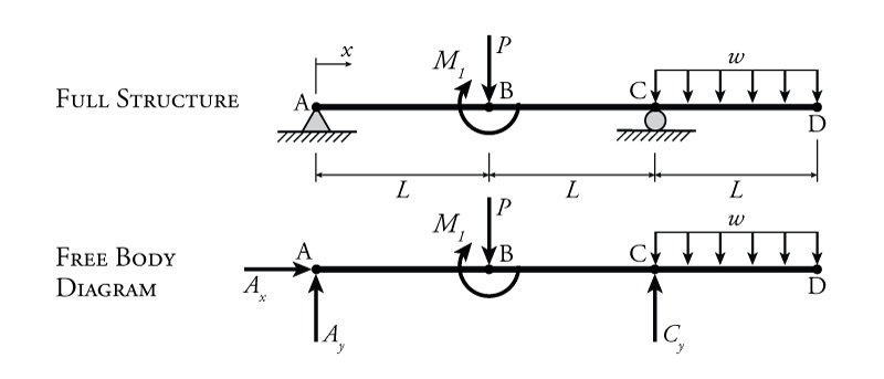
In the example structure shown in Figure 4.2, we will be treating the external point load $P$, the external distributed load $w$, and the external point moment $M_1$ as known external forces on the structure. For this example we will keep them in terms of $P$, $w$ and $M_1$ so that our solution is applicable to a wide range of different problems; however, these external forces could also have been given in absolute quantities instead of variables. For example, the point load could be $10\mathrm{\,kN}$ and distributed load could have a value of $20\mathrm{\,kN/m}$. Note that while the point load has units of force, the distributed load is in units of force per unit length (e.g. $20\mathrm{\,kN/m}$ distributed evenly on every meter of the beam's length). The reaction forces are unknown at the start of the problem, but since we are analysing a determinate beam, they may easily be found in terms of the external forces using equilibrium. Just like the external forces, the member length $L$ will also be treated as known. Note that members AB, BC, and CD all have the same length $L$.
Our ultimate goal in this problem is to find the internal shear forces and bending moments at every point along the beam in terms of the known external forces and known member lengths. This way, for any problem that looks like this one, we can just plug in the known external forces and lengths and immediately calculate the associated shears and moments.
Analysis using Section Cuts
To analyse the beam using cut free body diagrams, we must construct multiple FBDs, each one cut at one of the different conditions that we find on the beam (we will see what that looks like in a moment).
The first step is to find the reaction forces. For the example structure in Figure 4.2, we can use our equilibrium equations for 2D:
\begin{align*} \rightarrow \sum F_x &= 0 \end{align*} \begin{equation*} \boxed{A_x = 0} \end{equation*}
There is only one horizontal force ($A_x$) and so, therefore, it must be zero. This is common in beam problems. Then, using moment equilibrium about point A:
\begin{align*} \curvearrowleft \sum M_A &= 0 \\ -PL - M_1 + C_y (2L) - w(L)(2.5L) &= 0 \\ C_y(2L) &= PL + M_1 + 2.5wL^2 \\ C_y &= \frac{PL + M_1 + 2.5wL^2}{2L} \end{align*} \begin{equation*} \boxed{C_y = 0.5P + 1.25wL + \frac{0.5M_1}{L} \uparrow} \end{equation*}
The moment arm for the point load is simply $L$. For the vertical reaction $C_y$, the moment arm is $2L$ (the distance between points A and C). For the uniformly distributed load $w$, we calculate the moment by finding the total value of the distributed load (the distributed load per unit length times the length, giving $wL$), and then considering that that total load acts like an effective force $wL$ acting at the centre of the distributed load. This centre is $2.5L$ away from point A, giving the total moment $wL(2.5L)=2.5wL^2$. For the point moment $M_1$ there is no moment arm, point moments are always added as-is in moment equilibrium equations. In this case the point moment is negative since it is acting clockwise (see Section 1.6). Point moments do not effect horizontal or vertical equilibrium equations. Knowing $C_y$ now, we can find $A_y$ using vertical equilibrium:
\begin{align*} \uparrow \sum F_y &= 0 \\ A_y - P + C_y - w(L) &= 0 \end{align*}
Subbing in the known solution for $C_y$:
\begin{align*} A_y &- P + 0.5P + 1.25wL + \frac{0.5M_1}{L} - w(L) = 0 \\ A_y &= P - 0.5P - 1.25wL - \frac{0.5M_1}{L} + wL \\ \end{align*} \begin{equation*} \boxed{A_y = 0.5P - 0.25wL - \frac{0.5M_1}{L} \uparrow} \end{equation*}
Now that we have the reaction forces, we can make our section cuts to find equations for the internal shear and moment in the beam as a function of the location along the beam's length. Starting at the left, we need to make a new cut within every type of beam section. For this beam, we will cut once between points A and B, between points B and C, and between points C and D as shown in Figure 4.3. If there were additional external loads on the beam then we would have to ensure that there is a cut on each side of a location in the member where the loading or support condition changes. For example, if there was an additional point load between points B and C, we would have to cut BC twice, once to the left of the new point load and once to the right of it. Another way to think about this is that if you move from one side of the beam to the other, every time you pass a new external load or support, you need to make a new cut somewhere past it. Using the FBDs that result from each cut, we can find the internal shear and moment for each section of the beam as a function of the location $x$. For this example we have chosen $x=0$ to be the left end of the beam at point A (as shown by the unidirectional arrow labelled $x$ in Figure 4.2). Likewise, at point B: $x=L$, at point C: $x=2L$ and at point D: $x=3L$.
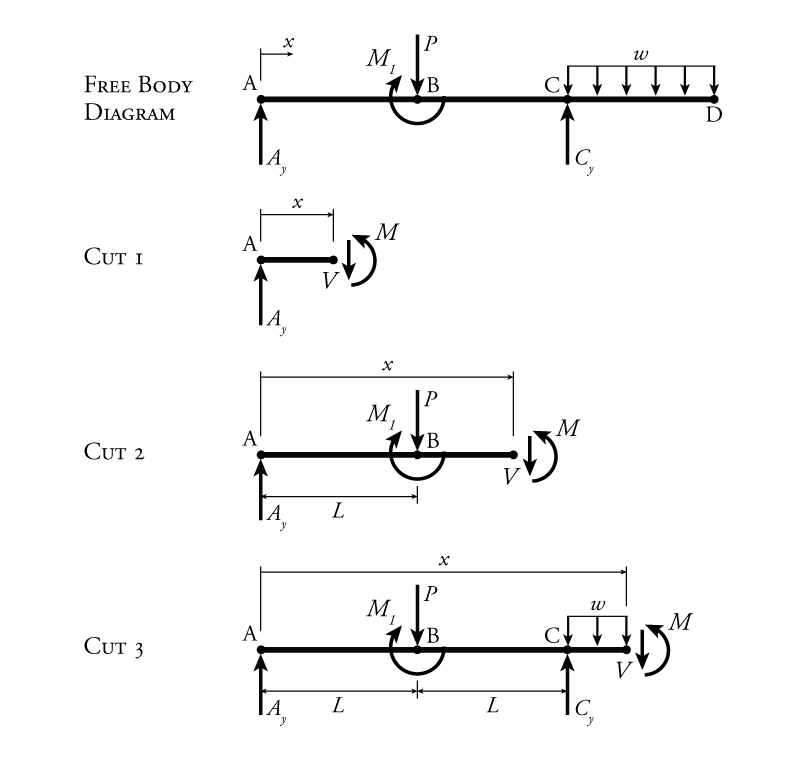
Every time we take a cut in a beam or frame member, we have an axial force, shear force and moment at the cut that represent the forces that are transmitted across the cut from one side to the other. In our example beam, we already know that we don't have axial force, so the only forces shown across the cuts in Figure 4.3 are the shear force and the moment. Since we know the reactions, we can easily use equilibrium to solve for the unknown shear and moment for each cut location. The only tricky part is that these shear forces and moments will be in terms of the distance along the beam $x$ (so the equations for shear and moment will be functions of $x$). This is because the equilibrium solution at the cut is valid for the whole section. For example, it doesn't matter where we cut member AB in this process, that cut represents the change in shear and moment everywhere between point A and point B.
It is also important to note that the unknown internal forces should be drawn in their positive sense (refer back to Section 1.6 for the sign conventions for internal shear and moment). Since we are applying the sign convention for internal forces, internal shear force is positive on the left end of a beam cut if the shear force arrow points upwards, and positive on the right side of beam cut if the shear force arrow points downwards. In this case, the shear is on the right side of a beam cut, so positive shear is down. The same applies to the moment sign convention; since we are looking at the right end of a beam cut, the moment arrow for positive moment must be counter-clockwise.
For Cut 1 in Figure 4.3, the unknown shear may be found using vertical equilibrium:
\begin{align*} \uparrow \sum F_y &= 0 \\ A_y - V &= 0 \\ V &= A_y \end{align*}
Since we already know $A_y$, we can say:
\begin{equation*} \boxed{\text{For } x<L: V = 0.5P - 0.25wL - \frac{0.5M_1}{L}} \end{equation*}
The location $x$ did not come into the vertical equilibrium, and so we know that the shear must be constant between points A and B. Similarly, the internal moment may be found using a moment equilibrium about the cut point:
\begin{align*} \curvearrowleft \sum M_{cut} &= 0 \\ M - A_y(x) &= 0 \\ M &= A_y x \end{align*} \begin{equation*} \boxed{\text{For } x<L: M = x \left[ 0.5P - 0.25wL - \frac{0.5M_1}{L} \right] } \end{equation*}
The moment $M$ is a linear function of $x$ (all the variables within the square brackets are actually constants), and so we know that $M$ varies linearly between points A and B. At point A (where $x=0$), the internal moment $M=0$. At point B (where $x=L$):
\begin{equation*} \text{For } x=L: M = 0.5PL - 0.25wL^2 - 0.5M_1 \end{equation*}
To complete the analysis, we must repeat the above process for the other two cut sections. For Cut 2 in Figure 4.3:
\begin{align*} \uparrow \sum F_y &= 0 \\ A_y - P - V &= 0 \\ V &= A_y - P \end{align*} \begin{equation*} \boxed{\text{For } L<x<2L: V = -0.5P - 0.25wL - \frac{0.5M_1}{L}} \end{equation*}
and
\begin{align*} \curvearrowleft \sum M_{cut} &= 0 \\ M &- A_y(x) + P(x-L) - M_1 = 0 \\ M &= A_y x - P(x-L) + M_1 \\ M &= x \left[ 0.5P - 0.25wL - \frac{0.5M_1}{L} \right] -Px + PL + M_1 \\ M &= 0.5Px - 0.25wLx - \frac{0.5M_1x}{L} - Px + PL + M_1 \end{align*} \begin{equation*} \boxed{\text{For } L<x<2L: M = -0.5Px - 0.25wLx - \frac{0.5M_1x}{L} + PL + M_1 } \end{equation*}
Note that if we use this new equation for $M$ and sub in $x=L$, we get:
\begin{equation*} \text{For } x=L: M = 0.5PL - 0.25wL^2 + 0.5M_1 \end{equation*}
This is almost the same as the previous solution for $x=L$ from Cut 1 except that it has a $+ 0.5M_1$ instead of $- 0.5M_1$. This is because of the point moment $M_1$ at point B which is included in the equilibrium if we cut to the right of point B, but not included if we cut to the left of it. The moment as a function of $x$ is discontinuous at a place where a point moment is applied. At point C (where $x=2L$):
\begin{equation*} \text{For } x=2L: M = - 0.5wL^2 \end{equation*}
For Cut 3 in Figure 4.3:
\begin{align*} \uparrow \sum F_y &= 0 \\ A_y &- P +C_y - w(x-2L) - V = 0 \\ V &= A_y - P + C_y - w(x-2L) \\ V &= 0.5P - 0.25wL - \frac{0.5M_1}{L} -P \\ &\;\; + 0.5P + 1.25wL + \frac{0.5M_1}{L} - wx + 2wL \end{align*} \begin{equation*} \boxed{\text{For } 2L<x<3L: V = 3wL - wx = w(3L-x)} \end{equation*}
At the very end of the cantilever on the right at point D (where $x=3L$), the internal shear $V = 0$. For the moment:
\begin{align*} \curvearrowleft \sum M_{cut} &= 0 \\ M &- A_y(x) + P(x-L) - M_1 - C_y(x-2L) + w(x-2L) \left( \frac{x-2L}{2} \right)= 0 \\ M &= A_y x - P(x-L) + M_1 + C_y(x-2L) - w(x-2L) \left( \frac{x-2L}{2} \right) \\ M &= x \left[ 0.5P - 0.25wL - \frac{0.5M_1}{L} \right] -Px + PL + M_1 \\ &\;\; +(x-2L) \left[ 0.5P + 1.25wL + \frac{0.5M_1}{L} \right] \\ &\;\; - (wx - 2wL)(0.5x-L) \\ M &= 0.5Px - 0.25wLx - \frac{0.5M_1x}{L} - Px + PL + M_1 \\ &\;\; +0.5Px +1.25wLx + \frac{0.5M_1x}{L} - PL - 2.5wL^2 - M_1 \\ &\;\; - 0.5wx^2 + wxL + wxL - 2wL^2 \\ M &= 3wLx - 4.5wL^2 - 0.5wx^2 \end{align*} \begin{equation*} \boxed{\text{For } 2L<x<3L: M = w(3Lx - 4.5L^2 - 0.5x^2)} \end{equation*}
At point C (where $x=2L$):
\begin{equation*} \text{For } x=2L: M = w(6L^2-4.5L^2 -2L^2) = -0.5wL^2 \end{equation*}
which is the same as the moment at $x = 2L$ for the previous cut. This is expected since the moment should be continuous in the beam at point C if there is no point moment at that location. This is a nice check on our calculations, since we expect the moment to be zero at the free end and it is. At point D (where $x = 3L$):
\begin{equation*} \text{For } x=3L: M = w(9L^2-4.5L^2 -4.5L^2) = 0 \end{equation*}
which we expect because there should not be any moment at a free end (unless there is a point moment at that location).
The solution for Cut 3 would have been much easier if we used the right side of the cut instead of the left. This alternate cut is shown in Figure 4.4.
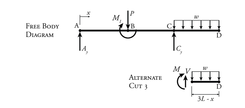
This cut is much easier to use to calculate the shear and moment because there are many less forces and reaction to take into account. Notice that the direction of the shear and moment at the cut have changed relative to the previous cuts. This is to maintain the positive internal force sign convention as shown in Section 1.6. Since we are now at the left end of a beam, positive internal shear points upwards and the positive internal moment is clockwise. To find the shear using vertical equilibrium:
\begin{align*} \uparrow \sum F_y &= 0 \\ V &- w (3L-x) = 0 \end{align*} \begin{equation*} \boxed{\text{For } 2L<x<3L: V = w(3L-x)} \end{equation*}
For the moment equilibrium about the cut end:
\begin{align*} \curvearrowleft \sum M_{cut} &= 0 \\ -M &- w(3L-x) \left( \frac{3L-x}{2} \right) = 0 \\ M &= (-3wL + wx)(1.5L - 0.5x) \\ M &= -4.5wL^2 + 1.5wLx + 1.5wLx - 0.5wx^2 \end{align*} \begin{equation*} \boxed{\text{For } 2L<x<3L: M = w(3Lx - 4.5L^2 - 0.5x^2)} \end{equation*}
Both of these are the same answers we got using the more difficult cut 3 FBD. The major benefit of doing it this way is that there are many fewer chances to make mistakes in the calculation. It is a common theme in structural analysis that we can save ourselves a lot of work if we think about the application of our methods and use them in a smart way.
Using the different section cuts, we were able to find the internal shear force and moment for every location along the beam as a function of $x$. This process would be simplified somewhat if we had used numerical values for the external forces and moments instead of the symbolic constants $P$, $w$ and $M_1$, but then our solution would have been less widely applicable.
If we assume a point load $P=20\mathrm{\,kN}$, a distributed load of $w=10\mathrm{\,kN/m}$, a point moment $M_1=30\mathrm{\,kNm}$ and a characteristic length $L=5\mathrm{\,m}$, then our shear and moment distributions would look like this:
\begin{align*} V(x) \left[ \mathrm{kN} \right] &= \left\{ \begin{array}{l l} -5.5 & \quad \text{if } x<L \\ -25.5 & \quad \text{if } L<x<2L \\ -10x+150 & \quad \text{if } 2L<x<3L \end{array} \right. \\ M(x) \left[ \mathrm{kNm} \right] &= \left\{ \begin{array}{l l} -5.5x & \quad \text{if } x<L \\ -25.5x+130 & \quad \text{if } L<x<2L \\ -5x^2 + 150x - 1125 & \quad \text{if } 2L<x<3L \end{array}\right. \end{align*}
Likewise, the reaction forces are:
\begin{align*} A_y = -5.5\mathrm{\,kN} = 5.5\mathrm{\,kN} \downarrow \\ C_y = 75.5\mathrm{\,kN} = 75.5\mathrm{\,kN} \uparrow \end{align*}
This example has shown that this section cutting method is quite time-consuming to use to find the shear and moments at every point in the beam (similar to the Method of Sections for truss analysis); however, it would be very easy to use a cut section to find the shear and moment at a specific single point in the beam (also similar to the Method of Sections). The results of this method may be used to draw shear force diagrams and bending moment diagrams for the beam. These simple diagrams are a key tool for structural engineers in design. They show a graphical representation of the distribution of the internal shear and moment in a beam.
The next section will introduce a simple graphical method which will allow us to draw the shear and bending moment diagrams for beams directly without the need for so much algebraic manipulation.
Graphical Integration
If you need to solve for the shear and moments at every point on a beam, it is often easier to use the graphical integration method. This method eliminates the need for finding the equations of shear and moment as a function of $x$ in most cases. This is useful, because in design, structural engineers are usually most concerned with either the maximum values of the shear and moment, or the value of shear and moment at a specific point along the beam only.
This graphical integration method is based on the simple but powerful relationships between the external load, shear force, and bending moment in a beam. Recall from mechanics:
\begin{align} \frac{dV(x)}{dx} &= w(x) \label{eq:shear-diff} \tag{1} \\ V(B) - V(A) &= \int_A^B w(x) \, dx \label{eq:shear-int} \tag{2} \\ \frac{dM(x)}{dx} &= V(x) \label{eq:moment-diff} \tag{3} \\ M(B) - M(A) &= \int_A^B V(x) \, dx \label{eq:moment-int} \tag{4} \end{align}
where $w(x)$ is a general expression for the distributed load on the beam as a function of the location $x$ along the beam, $V(x)$ is the internal shear as a function of $x$ and $M(x)$ is the internal bending moment as a function of $x$.
The results of a graphical integration analysis are a shear force diagram and a bending moment diagram (often called a BMD). These diagrams are effectively plots of the functions $V(x)$ and $M(x)$, respectively, with the horizontal axis representing the length along the beam $x$. This is convenient because it means that we can effectively draw these diagrams right over-top of a drawing of the beam itself.
The consequence of equation \eqref{eq:shear-diff} is that the slope of the shear force diagram at any particular location $x$ is equal to the value of the distributed load $w$ (in units of force per unit distance) at that location. Equation \eqref{eq:shear-int} was found by integrating equation \eqref{eq:shear-diff} with the limits of integration $x=A$ and $x=B$. The consequence of equation \eqref{eq:shear-int} is that the total area under the distributed load between points A and B is equal to the change in the shear force between those two points. This area under the distributed loads may be found using the equivalent total loads shown previously in Section 4.2. The relationship between applied load and internal shear force may be rephrased as follows: the shear force at any point along a beam is equal to the cumulative sum of the area under the distributed loads along the length of the beam up to that point.
Point loads act at only a single point on a beam or frame member. Therefore, the 'area' under the point load is simply the magnitude of the point load itself. This means that a point load will cause an instantaneous jump (or step) in the shear force at the point where it is applied. This is true whether the point load is caused by an external load or by a reaction force. The structure cannot distinguish between external forces and reactions, they are both just forces from it's point of view. In a practical sense, the only difference between the two to an engineer is that we usually know the external forces, but need to calculate the reactions.
Similar to the relationship between shear force and distributed load, an equivalent relationship exists between the moment and the shear force. As equation \eqref{eq:moment-diff} shows, the derivative of the moment at any point is equal to the shear force at that point. This means that the slope of the moment diagram at at any particular location $x$ (in units of force multiplied by length) is equal to the value of the shear force $V(x)$ (in units of force) at that location. Equation \eqref{eq:moment-int}was found by integrating equation \eqref{eq:moment-diff} with the limits of integration $x=A$ and $x=B$. The consequence of equation \eqref{eq:moment-int} is that the total area under the shear force diagram between points A and B is equal to the changein the moment diagram between those two points. Or, rephrased, the bending moment at any point is equal to the cumulative sum of the area under the shear force diagram along the length of the beam up to that point.
The situation for a point moment is similar to the situation for a point load. A point moment causes an instantaneous jump or step in the bending moment diagram. A point moment will not affect the shear force diagram.
Given all of these relationships between area of one diagram and the change in the value of another, you can see how we can start with a given loading profile on a beam (distributed loads and point loads caused by external forces and reactions) and use those loadings to determine the shear force diagram by summing up the areas under the loads starting at one end of the beam and moving towards the other. Then, once we have the shear force diagram, we can use the same method to sum up the areas under the shear force diagram to find the resulting bending moment diagram.
This process of graphical integration may be summarized into the following steps:
- Use equilibrium to find all reaction forces.
- Use the resulting loading profile to construct the shear force diagram as follows.
- Start from the left end of the beam and move towards the right end.
- For each point load that is encountered, change the shear force diagram value by the value of the point load at that location (increase shear force for an upwards force and decrease shear force for a downwards force).
- If there is no external force (or reaction) along a portion of the beam, keep the shear force constant for that portion.
- For a portion of the beam with a distributed load, find the total force caused by the full distributed load. At the right end of the distributed load, the shear force will be equal to the shear force at the left of the distribution added to the total force caused by the distributed load. For distributed loads that point up, the total load should be added to the shear, and for distributed loads that point down, the total load should be subtracted from the shear. The line connecting the two ends of the distribution on the shear force diagram will have a different shape depending on the type of distribution. For a uniform distribution, it will be a straight line. The easy way to determine the shape of the shear diagram between the two ends is to remember that the slope of the shear force diagram is equal to the value of the distributed load at any point. Since a uniform load has a constant value along the distribution, the slope of the shear force diagram is constant (i.e. a straight line). For more complex distributions, it can help to draw the slope of the shear force diagram at either end of the distribution and then connect the two ends with a curve. A triangular or trapezoidal load distribution will result in a parabolic shape between the two ends on the shear force diagram (because in integral of a line is a parabola).
- Point moments will not affect the shear force diagram.
- When you get all the way to the other end of the beam, the shear force diagram should return to zero. This does not mean that the value of the shear is zero at the end, because it is often a point load that brings the shear back to the horizontal axis. In such a case, the value of the shear at the end of the beam is equal to the value of the point load.
- Use the resulting shear force diagram to construct the bending moment diagram.
- Divide the shear force diagram into sections so that each section is a simple shape.
- Again, start from the left end of the shear force diagram and move towards the right end.
- If there is no shear force along a section of the beam, keep the moment diagram constant for that section.
- For each section of the shear force diagram, find the total area of that section. At the right end of the section, the moment will be equal to the moment at the left side of the section plus the total area under the shear force diagram between the two ends. Positive shears should be added, and negative shears should be subtracted. The line connecting the two ends of the section on the moment diagram will have a different shape depending on the shape of the shear force diagram. For a constant shear, it will be a straight line. Again, the easy way to determine this is to remember that the slope of the moment diagram is equal to the value of the shear force diagram at any point. Hence, if the shear force diagram has a constant value along the distribution, the slope of the moment diagram diagram is constant (i.e. a straight line). For more complex distributions, it can help to draw the slope of the moment diagram at either end of the section and then connect the two ends with a curve. A triangular or trapezoidal shape on the shear force diagram will result in a parabolic shape between the two ends of the section on the moment diagram. A parabolic shear force diagram will result in a cubic moment diagram.
- At the same time, as you are going along the beam, every point moment (found on the loading profile) will change the moment diagram value instantaneously at that point by the value of that point moment at that location.
If you move from left to right across the beam, a clockwise moment will cause the moment diagram to jump upwards and a counter-clockwise moment will cause the moment diagram to jump downwards. This is the opposite of what you might expect since we generally consider clockwise moments to be negative.
- By the time you get to the other end of the beam, the moment diagram should return to zero. Again, this does not mean that the value of the moment is zero at the end (although it often is). Sometimes a point moment at the end (from a fixed reaction for example) brings the moment back to the horizontal axis. In such a case, the value of the moment at the end of the beam is equal to the value of the point moment reaction.
This process will now be illustrated using the same example from the previous section (Figure 4.2). For this example, we will use the same assumed values for the point load of $P=20\mathrm{\,kN}$, distributed load of $w=10\mathrm{\,kN/m}$, point moment of $M_1=30\mathrm{\,kNm}$ and characteristic length of $L=5\mathrm{\,m}$. Using these values, the reaction forces are calculated in the same way as before to be:
\begin{align*} A_y = -5.5\mathrm{\,kN} = 5.5\mathrm{\,kN} \downarrow \\ C_y = 75.5\mathrm{\,kN} = 75.5\mathrm{\,kN} \uparrow \end{align*}
The resulting free body diagram for the system is shown at the top of Figure 4.5.
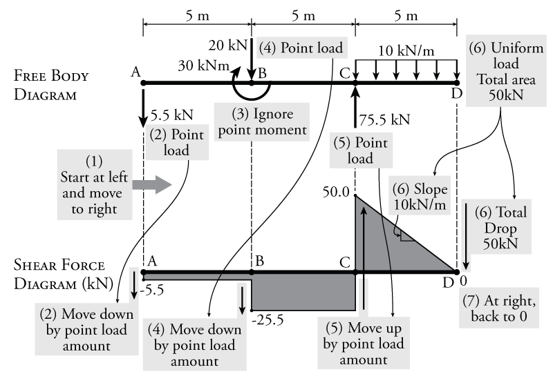
From the free body diagram, we can immediately start to draw the shear force diagram as illustrated in Figure 4.5:
- Start from the left side of the beam and progress towards the right, including each load (point or distributed) that is encountered along the way.
- The first load is a point load at A (the reaction $A_y$). The load is pulling down. Therefore, starting at 0 on our shear force diagram at point A, we move down by the value of the point load ($5.5\mathrm{\,kN}$). As we move rightwards past point A, there are no loading effects until point B, so the shear force remains constant at the same level until then.
- The next load is the point moment at point B; however, point moments do not affect the shear force in the beam, so we will ignore this for now (it will have to be considered when we construct the moment diagram).
- There is also a vertical point load at B which pushes down on B. Therefore, starting at our previous value ($-5.5\mathrm{\,kN}$) we move down by an additional amount equal to the value of the point load ($20\mathrm{\,kN}$). This results in a total shear force just to the right of point B of $-5.5-20=-25.5\mathrm{\,kN}$. Again, between points B and C, the shear force remains constant.
- At point C, there is another vertical point load (the reaction $C_y$) which pushed the beam upwards. Therefore, again starting at our previous value ($-25.5\mathrm{\,kN}$), we move up (add) the value of the point load ($75.5\mathrm{\,kN}$). This results in a total shear force just to the right of point C of $-25.5+75.5=+50.0\mathrm{\,kN}$.
- Between points C and D, there is a uniformly distributed load of $10\mathrm{\,kN/m}$ pushing the beam downwards. This distributed load steadily moves the shear force diagram down by $10\mathrm{\,kN}$ for every metre of beam length. This is equivalent to a line on the shear force diagram that starts at the previous shear value of $50\mathrm{\,kN}$ and has a negative slope of $-10\mathrm{\,kN/m}$ until it reaches point D. Notice that the slope of the shear force diagram is equal to the value of the distributed load as previously discussed. The total drop in the shear force over the section from point C to point D is equal to the area under the distributed load which is equal to $10(5)=50\mathrm{\,kN}$.
- By the time the shear force diagram reaches the end of the beam at point D (and there are no additional loads to consider at point D for this example), the shear force diagram has come back to 0, which is expected. If it does not come back to zero, than there is likely some error in your calculation.
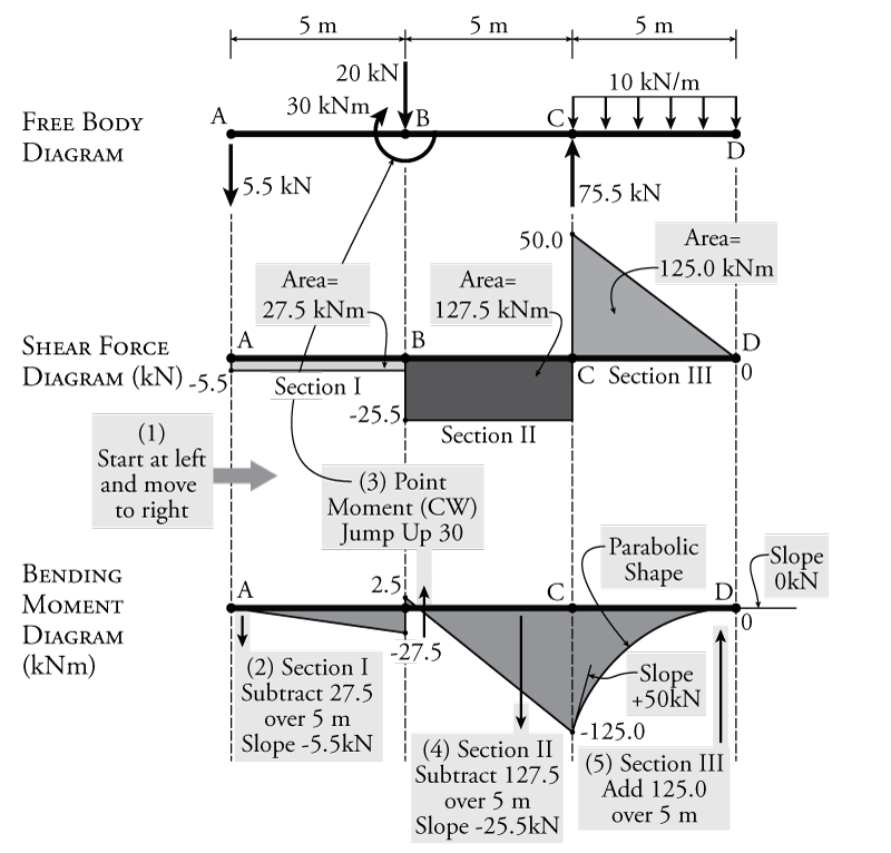
Now that we have constructed the shear force diagram, we can continue and construct the bending moment diagram for the beam as illustrated in Figure 4.6:
- The shear force diagram has been divided into three sections as shown in the figure. Each section is a simple shape (Section I and II are rectangles and Section III is a triangle), and the area of each section is shown. Similarly to when we constructed the shear force diagram, start from the left side of the beam and progress towards the right, including each section of the shear force diagram along the way (also making sure not to forget to include any point moments from the free body diagram).
- For each section of the shear force diagram, the total change in the moment diagram between the left end of the section and the right end is equal to the area of the shear force diagram section. For Section I (which is between points A and B), the total area is $-27.5\mathrm{\,kNm}$ (negative because the area lies below the horizontal axis). So the total drop in the moment diagram between points A and B is equal to $-27.5\mathrm{\,kNm}$. Similar to the construction of the shear force diagram, the slope of the moment diagram at any point is equal to the corresponding value of the shear force diagram at that point. Since the shear force diagram has a constant value ($-5.5\mathrm{\,kN}$) between points A and B, the slope of the moment diagram is also constant between points A and B and equal to $-5.5\mathrm{\,kN}$.
- At point B, there is a point moment on the free body diagram. Since that point moment is clockwise, it creates a positive instantaneous jump in the bending moment diagram at point B. The amount of this jump is equal to the value of the point moment ($30\mathrm{\,kNm}$) and is relative to the previous value of the moment diagram at that location (we were at $-27.5\mathrm{\,kNm}$ due to the shear between points A and B). Don't forget that the direction of this jump is backwards with respect to our normal sign convention for moments (which is counter-clockwise positive).
- For Section II (which is between points B and C), the total area is $-127.5\mathrm{\,kNm}$, resulting in a total drop in the bending moment diagram of the same amount. For this section, the value of the shear force diagram is also constant, and so the slope of the moment diagram is also constant and equal to $-25.5\mathrm{\,kN}$ which is steeper than the slope for Section I.
- For the last section, Section III (which is between points C and D), the shear force is not constant. It varies linearly from $50\mathrm{\,kN}$ at point C to zero at point D. The total area of that section ($125.0\mathrm{\,kNm}$) is still equal to the total rise between points C and D, and we can see that the bending moment diagram will end at zero by point D as we expect; however, the shape of the bending moment diagram will no longer be linear. Since the value of the shear force changes, so does the slope of the moment diagram. At point C, the shear force (and, hence, the slope) is equal to $+50\mathrm{\,kN}$ as shown by the tangent line in the figure. At point D, the shear force (slope) is equal to 0, or a horizontal line as shown. An easy way to draw the bending moment diagram between points C and D is to first find the end points (using the area of the shear force diagram to calculate the total rise or drop) and then draw in the approximate slope at each end using the value of the shear force diagram. A curve can then be drawn to join the two points with the appropriate end slopes. We know that the moment diagram curve should look like a parabola since the shear force diagram curve was linear (recall that if you integrate a straight line, you get a parabola). Likewise, if the shear diagram had a parabolic shape, the moment diagram should have the shape of a third-order polynomial (which will still look similar to a parabola).
By this point, the full shear and bending moment diagrams have been constructed and drawn. After getting some practice using this method, you will find that you are able to draw shear force and bending moment diagrams very quickly for any loading conditions. You can check yourself to see that we got the same answer using this method as we did using the section cutting method that we used previously.