 Learn About Structures
The construction of influence lines for trusses is similar to the construction of influence lines for beams; however, as mentioned previously, it is important to determine which path the moving load takes across the truss. An example truss for a road bridge is shown in Figure 6.11. On this truss, the road surface is level with the lower chord of the truss. Therefore, an influence line for this truss would be constructed along a direct line that joins the pin at the left with the roller on the right along the lower chord of the truss.
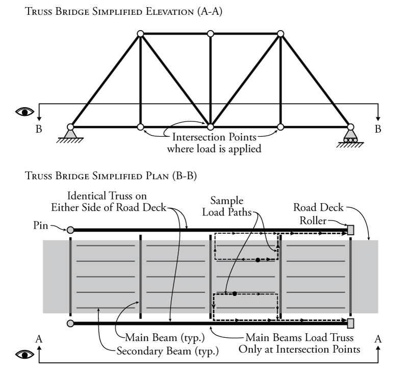
Another important difference for influence lines for trusses is that we must assume that the load can only be transferred to the truss at the intersection points between the members. This is necessary because the truss members themselves are often assumed in design to only take axial forces. Any loads between the intersection points on the truss elements would cause them to bend. This is also how real trusses are often designed as shown in Figure 6.11. In the figure, a typical simply-supported truss bridge is shown at the top. Of course, for a bridge, you need to actually have two trusses, one on either side of the roadway. This is shown in the plan at the bottom of the figure, where the road deck is shown by the grey shaded area and the trusses are on either side (top and bottom). These trusses are joined together by main beams that run between them at the locations of the intersection points between the truss members. These main beams are responsible for transmitting the load from the roadway to the truss intersection points. The main beams are also often connected together by secondary beams. The road deck would then sit on top of the secondary beams. So, the load path for a load applied on any point of the road deck must travel through the secondary beams to the closest main beam, and from there directly to an intersection point on the truss. The truss then transfers the main beam loads from the intersection points to the supports at either end. Sample load paths are shown in Figure 6.11.
This means that any load that is located between intersection points will be split between the two closest intersection points (in proportion to how close the load is to each intersection point). This means that in between the intersection points, the values are just an interpolation between the two closest points. For truss influence lines, the consequence of this is that we can find the values for the influence line at the at intersection points, and then just connect the points together using straight lines.
To find these influence lines, there is no easy Müller-Breslau principle. The method of joints or method of sections must be used to find a truss member force as a function of the moving unit load position. This also means that, like the equilibrium method for beams, you often must find the influence diagrams for one or more reaction forces before you can find the influence diagram for the internal axial force in a specific truss member.
Example
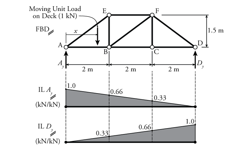
An example truss is shown in Figure 6.12. This truss supports a bridge and the deck of the bridge is concurrent with the bottom chord of the truss. So, the path for the moving unit point load is along a line joining points A and D. The distance $x$ is the distance of the moving load from point A. Find the influence lines for the three members EF, BF and BC.

To find those member influence lines, we first have to find the influence lines for the reactions at A and D (IL $A_y$ and IL $D_y$). Since we can use external equilibrium to find the reactions, the process of finding reaction influence lines for trusses is the same as it was for beams. For the influence on reaction at $D_y$ we can use a moment equilibrium about point A:
\begin{align*} \curvearrowleft \sum M_A &= 0 \\ (-1.0)x + D_y(6) &= 0 \end{align*} \begin{equation*} \boxed{D_y = \frac{x}{6}} \end{equation*}
And vertical equilibrium for the influence line for the reaction at point A:
\begin{align*} \uparrow \sum F_y &= 0 \\ A_y -1.0 + D_y &= 0 \\ A_y -1.0 + \frac{x}{6} &= 0 \end{align*} \begin{equation*} \boxed{A_y = 1.0 - \frac{x}{6}} \end{equation*}
These resulting influence lines are shown in Figure 6.13.
Now that we know the influence line expressions for the reactions, we can use the method of sections to find the influence diagrams for the internal axial forces in members EF, BF and BC. The free body diagrams for the left and right cuts to find those internal forces are shown at the top of Figure 6.14; however, the solution to this problem is more complex because there are three different possible locations for the moving point load: on the left side of the cut between A and B, on the right side of the cut between C and D, and between the two sides of the cut between B and C. The point load being located in each of these different locations will affect the equilibrium of the cut sections differently. Therefore, we have to consider all three cases for each influence diagram that we want to construct.
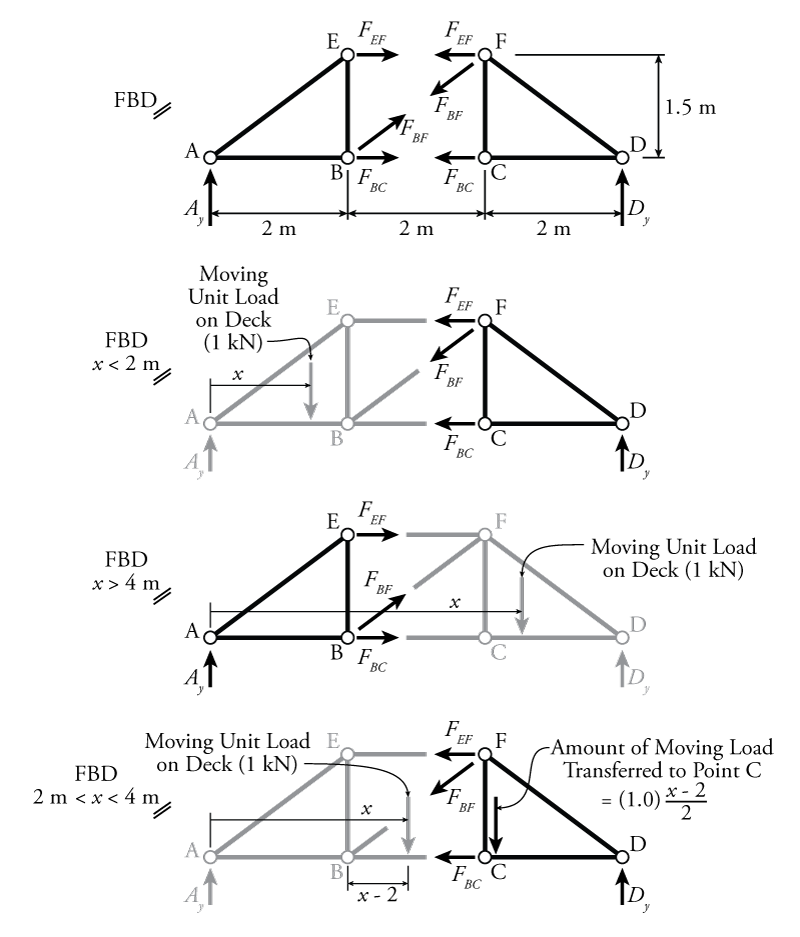
Of course, for the solution of any particular internal member axial force, we can use equilibrium on either side of the cut. But, to make our lives easier, it is typically simpler to select whichever side of the cut does not have the moving unit point load on it. So, when the point load is located on the left side of the cut between A and B ($x<2$), it simplifies the analysis to find the forces in the cut members using the right side section. Likewise, when the point load is located on the right side ($x>4$), it makes sense to do the equilibrium calculations using the left side section. These two situations are shown in the middle two diagrams in Figure 6.14. When the moving point load is between the two cut sections (between B and C, $2 < x < 4$), it doesn't matter which side cut section you use because some portion of the load in between B and C will be transferred to the closest intersection point as shown on the bottom diagram of Figure 6.14.
Let's start with the influence diagram for the axial force in member EF ($F_{EF}$). The first case we will consider is for when the moving point load is on the left section ($x<2$). To solve for $F_{EF}$ we will use equilibrium on the right section as shown in the second diagram from the top in Figure 6.14. If we use the right section, the moving point load itself will not come into the equilibrium calculation as shown. To find $F_{EF}$ we can use a moment equilibrium about point B. This is okay even though point B is not part of the section. It is just a convenient point in space that is concurrent with forces $F_{BF}$ and $F_{BC}$ so that those two forces will not come into the moment equilibrium calculation.
\begin{align*} \curvearrowleft \sum M_B &= 0 \\ D_y(4) + F_{EF}(1.5) &= 0 \\ F_{EF} &= - \frac{8}{3} D_y \end{align*}
but we know from our previous reaction influence line calculations that:
\begin{align*} D_y &= \frac{x}{6} \\ \text{so, } F_{EF} &= - \frac{8}{3} \left( \frac{x}{6} \right) \end{align*} \begin{equation*} \boxed{F_{EF} = -\frac{4x}{9} \; \text{for} \; x < 2} \end{equation*}
For the same force $F_{EF}$, when the unit point load is on the right section ($x>4$), we will use equilibrium on the left section as shown in the third diagram from the top in Figure 6.14. Again, using moment equilibrium about point B:
\begin{align*} \curvearrowleft \sum M_B &= 0 \\ -A_y(2) - F_{EF}(1.5) &= 0 \\ F_{EF} &= - \frac{4}{3} A_y \end{align*}
but we know from our previous reaction influence line calculations that:
\begin{align*} A_y &= 1.0 - \frac{x}{6} \\ \text{so, } F_{EF} &= - \frac{4}{3} \left( 1.0 - \frac{x}{6} \right) \end{align*} \begin{equation*} \boxed{F_{EF} = -\frac{4}{3}+\frac{2x}{9} \; \text{for} \; x > 4} \end{equation*}
When the moving unit load is in between the two sections ($2<x<4$), then some portion of the moving load will be transferred to the joint closest to the section. If we use the equilibrium on the right section (as shown in the bottom diagram of Figure 6.14), then the portion of the moving point load that is transferred to point C is dependent on how close the point load is to point C (relative to point B). In the figure, the distance between the moving point load and point B is $x-2$. The corresponding resulting load on point C caused by the unit load is equal to:
\begin{align*} (1.0) \frac{x-2}{2} \end{align*}
So, when the point load gets to C ($x = 4$), then the load on C will be equal to 1.0. When the load is at B ($x = 2$) the load on C will equal 0. Including this transferred load in the equilibrium of the right side of the cut as shown in the lower diagram of Figure 6.14, we can again use the moment equilibrium about point B:
\begin{align*} \curvearrowleft \sum M_B &= 0 \\ D_y(4) - (1.0) \frac{x-2}{2} (2) + F_{EF}(1.5) &= 0 \\ (1.5) F_{EF} &= \frac{x}{3} - 2 \end{align*} \begin{equation*} \boxed{F_{EF} = \frac{2x}{9} - \frac{4}{3} \; \text{for} \; 2 < x < 4} \end{equation*}
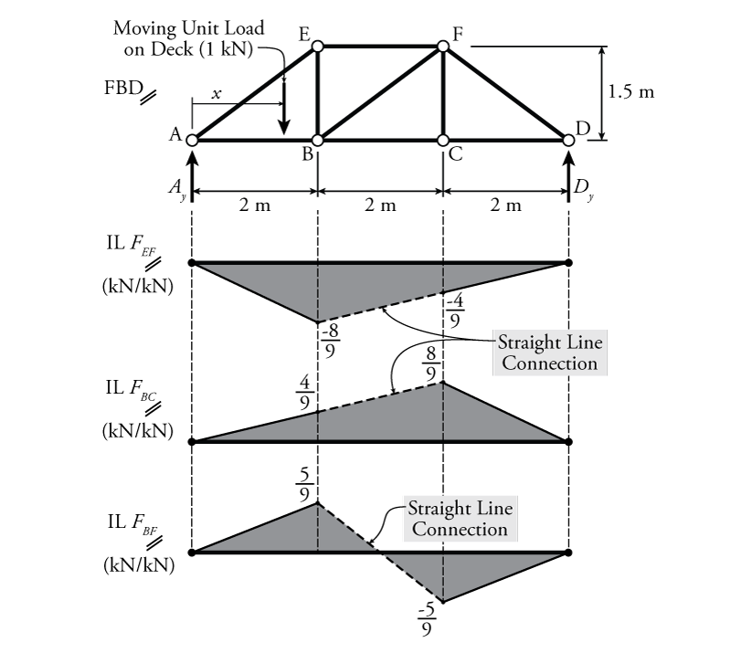
At this point we have found the value of the influence line for every potential location of the point load ($x<2$, $2<x<4$, and $x>4$). The resulting influence line is shown in Figure 6.15 (IL $F_{EF}$). We can draw these easily by simply drawing the end point for each section and connecting the end points with straight lines. For example, for the section $x<2$ we can find the $F_{EF}$ for $x = 0$ and $x=2$ and join the area between the two points with a straight line.
As discussed previously, the influence lines for determinate trusses consist of straight lines and that those lines are interpolations between the influence line values at the intersection points. Therefore, although we explicitly solved for all three potential ranges of $x$, we could have just solved only for the situations where the point load is on the left of the cut and the right of the cut ($x<2$, and $x>4$). If we did that, and drew the influence lines for those portions, we can find the influence line for the section in between the cuts by simply drawing a straight line between the values at the edges of the cut as shown in Figure 6.15. This saves the trouble of having to consider the portion of the moving unit load in between the cut sections that acts on the equilibrium section.
Using the same method, we can find influence lines for the other internal axial forces in members BC and BF. For member BC ($F_{BC}$), when $x<2$, use the right side cut section from Figure 6.14 and a moment equilibrium about point F:
\begin{align*} \curvearrowleft \sum M_F &= 0 \\ D_y(2) - F_{BC}(1.5) &= 0 \\ F_{BC} &= \frac{4}{3} D_y \end{align*} \begin{equation*} \boxed{F_{BC} = \frac{2x}{9} \; \text{for} \; x < 2} \end{equation*}
For member BC ($F_{BC}$), when $x>4$, use the left side cut section from Figure 6.14 and a moment equilibrium about point F:
\begin{align*} \curvearrowleft \sum M_F &= 0 \\ -A_y(4) + F_{BC}(1.5) &= 0 \\ F_{BC} &= \frac{8}{3} A_y \end{align*} \begin{equation*} \boxed{F_{BC} = \frac{8}{3} - \frac{4x}{9} \; \text{for} \; x > 4} \end{equation*}
The resulting influence line for the axial force in member BC (IL $F_{BC}$) is shown in Figure 6.15. This time, since we didn't find the expression for the influence line between B and C explicitly, we can just connect the influence diagrams for the left and right sides using a straight line as shown in the figure.
Lastly, for the influence diagram of the force in member BF ($F_{BF}$), when $x<2$, use the right side cut section from Figure 6.14 and a vertical equilibrium:
\begin{align*} \uparrow \sum F_y &= 0 \\ D_y - F_{BF}\left( \frac{1.5}{2.5} \right) &= 0 \\ F_{BF} &= \frac{5}{3} D_y \end{align*} \begin{equation*} \boxed{F_{BF} = \frac{5x}{18} \; \text{for} \; x < 2} \end{equation*}
For member BF ($F_{BF}$), when $x>4$, use the left side cut section from Figure 6.14 and vertical equilibrium:
\begin{align*} \uparrow \sum F_y &= 0 \\ A_y + F_{BF}\left( \frac{1.5}{2.5} \right) &= 0 \\ F_{BF} &= -\frac{5}{3} A_y \end{align*} \begin{equation*} \boxed{F_{BF} = \frac{5x}{18} - \frac{5}{3} \; \text{for} \; x > 4} \end{equation*}
Again, the resulting influence line for the axial force in member BF (IL $F_{BF}$) is shown in Figure 6.15, and we can just connect the influence diagrams for the left and right sides using a straight line as shown in the figure.