 Learn About Structures
In his own words, Hardy Cross summarizes the moment-distribution method as follows:
The method of moment distribution is this: (a) Imagine all joints in the structure held so that they cannot rotate and compute the moments at the ends of the member for this condition; (b) at each joint distribute the unbalanced fixed-end moment among the connecting members in proportion to the constant for each member defined as "stiffness"; (c) multiply the moment distributed to each member at a joint by the carry-over factor at that end of the member and set this product at the other end of the member; (d) distribute these moments just "carried over"; (e) repeat the process until the moments to be carried over are small enough to be neglected; and (f) add all moments -- fixed-end moments, distributed moments, moments carried over -- at each end of each member to obtain the true moment at the end
Cross, H. (1949) Analysis of Continuous Frames by Distributing Fixed-End Moments. Transactions of the American Society of Civil Engineers, Vol. 96, No. 1, January 1932, pp. 1-10}).
So this method amounts to first assuming each joint is fixed for rotation (locked). Then by locking and unlocking each joint in succession, the internal moments at the joints are slowly distributed and balanced until each joint reaches a final equilibrium condition. We will see this process in detail through the use of an example is a later section.
The generalized moment distribution method procedure is illustrated in Figure 10.2. Parts of this figure, referenced by part letter will be referenced in the description below. To picture the moment distribution method conceptually, imagine that at the start of our analysis, before we even add any external loads to the structure, we grab hold of all of the nodes and prevent them from rotating (b). This effectively causes the ends of all the members to be fixed. Then, we apply all of the external loads on the structure (c). Those external loads on the members cause a moment at each fixed end, which we can calculate (d). Then, for each node in turn, one at a time, we can unlock the node and then lock it up again (e). The act of unlocking the node allows that node to rotate freely. This rotation is caused by whatever unbalanced moment there is on the node prior to the unlocking. Unbalanced loads are possible because the node was previously fixed, so one member connected to that node may be applying a fixed end moment to the node and another member connected to that node may be applying a different fixed end moment or none at all. These moments do not have to be in equilibrium prior to the unlocking because they are consider to be transferred not to the node, but to some external rotational support. Once we release the node, the node must rotate until it is in equilibrium. So, the total unbalanced moment present on the node before it is unlocked will be applied to the members that are attached to the node. Since all of the member ends that are connected to the node must rotate by the same amount when the node is released, the unbalanced moment will be distributed in proportion to the bending stiffness of each attached member (i.e. stiffer members take more moment for the same amount of rotation).
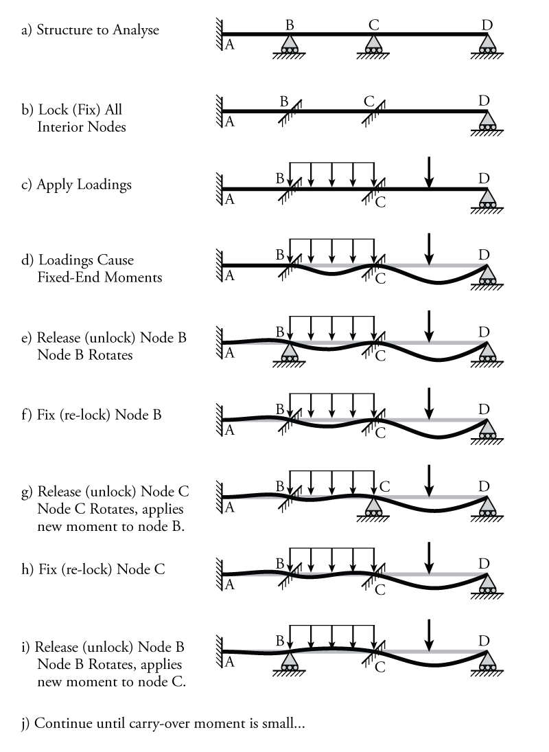
This act of applying moments to the members at the node also causes moments at the opposite ends of the members if they are fixed (the moment 'carries over' to the opposite end of the member). Once the node is in equilibrium, we lock it again (f), preventing it from rotating any further.
From here, we move on to the next node (g). When we look at the unbalanced moment at that node, we have to consider the moment caused by the fixed end forces in addition to any load that was carried over to that second node when the first node was released and then locked again. It is likely that for most structures each node will have to be locked and unlocked multiple times since unlocking one node may cause new unbalanced moments on other nodes that we have previously unlocked, balanced and then re-locked (h - j). This is why the moment distribution method is considered to be an iterative method. With enough iterations, though, we can eventually converge on the correct solution.
The key to this method is that, for the release of one node, we can easily calculate the proportion of the unbalanced moment needs to be apportioned to each connected member as well as how much moment should be carried over to the opposite end of the member. Since these are simple cases with few degrees-of-freedom, we can determine these using the previous methods that we have learned and then apply the results to all moment distribution method analyses. By only focusing on a limited part of the more complex structure in each step, we can analyse the structure piecemeal, without the need to directly solve a large system of simultaneous equations.
Each of the required components for a moment-distribution analysis, as introduced in the passage above, will be described in the following sections.
Sign Convention
The sign-convention for the moment distribution method is the same as the sign convention for the slope-deflection method, all counter-clockwise moments are considered positive and clockwise moments are considered negative. There is no consideration of the internal moment sign convention. All moments that are considered are point moments at member ends.
Fixed End Moments
In addition, the moment distribution method makes use of fixed end moments, just like the slope deflection method. To find fixed end moments, use the same figure (Figure 9.6) from Chapter 9.
Since we 'lock' all of the joints at the beginning of a moment distribution analysis, the fixed end moments represent the moments that each member applies to a locked node. These moments are caused by external forces on the structure that are applied between the member end nodes.
Member Stiffness and Carry-Over Factors
The key step of the moment-distribution method is the unlocking of each node and the redistribution of the unbalanced moment at that joint to all the members that are connected to it, based on relative rotational stiffness of each member. So, we need to be able to calculate the rotational stiffness of a member connected to a rotating joint, which will depend on the Young's modulus $E$, the moment of inertia $I$ and the length of the member. Like the slope-deflection method from Chapter 9, we would also like to take advantage of the extra information provided by pinned ends if we can, since we know ahead of time that the moment at such pinned ends must be zero. Hardy Cross's original method as described in the original paper does not take advantage of such additional information, but it will save us time and effort to do so. This means that the stiffness will also depend on the type of boundary condition at the opposite end of the member, whether it is fixed or pinned. Note that the pinned end condition only applies to pinned ends where the moment is zero.
When we redistribute the moment to the connected members at an unlocked node, the act of applying a moment to the end of a member connected to the node will also cause a moment at the opposite end of that member (unless the opposite end is pinned). These 'carried over' moments will need to be included in the calculation of the unbalanced moment at the opposite end node. So we must also determine how much of the moment is carried over.
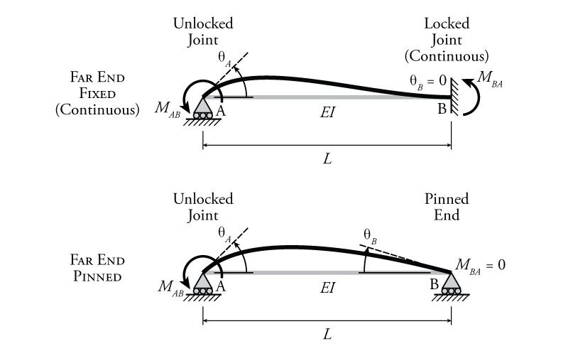
To determine the stiffness of a member connected to a node as well as the carried over moment, we can use the slope-deflection method from Chapter 9. For the case where the far end of the member is fixed, the member geometry and loading are shown at the top of Figure 10.3.
Recall that the slope-deflection equation for a single element is:
\begin{equation} M_{nf} = \frac{2EI}{L} (2 \theta_n + \theta_f - 3 \psi ) + \text{FEM}_{nf} \tag{1} \end{equation}
where node $n$ which is the node at the near end (the end that you are finding the end moment for) and node $f$ is node at the far end (the node at the opposite end of the element). So, the expression for $M_{AB}$ as shown in Figure 10.3 is:
\begin{align} M_{AB} = \frac{2EI}{L} (2 \theta_A + \theta_B - 3 \psi_{AB} ) + \text{FEM}_{AB} \tag{2} \end{align}
If the far end is fixed, as shown, then $\theta_B = 0$. In addition, there are no loads applied between the end nodes and there is no chord rotation, so $\text{FEM}_{AB}=0$ and $\psi_{AB}=0$. Including all of this, the expression for $M_{AB}$ becomes:
\begin{equation} \boxed{ M_{AB} = \frac{4EI}{L} \theta_A } \label{eq:Far-Fix-Near-Moment} \tag{3} \end{equation}
Rotational stiffness is the amount of moment required to rotate something by a unit amount of rotation, so:
\begin{align} k = \frac{M}{\theta} \tag{4} \end{align}
where $k$ is the rotational stiffness, $M$ is the moment, and $\theta$ is the rotation. For our system, we need to know the rotational stiffness of member AB, i.e. how much moment at node A on member AB is required to cause a one unit rotation at node A:
\begin{align} k_{AB} = \frac{M_{AB}}{\theta_A} \tag{5} \end{align}
From equation \eqref{eq:Far-Fix-Near-Moment}, we can see that:
\begin{equation} \frac {M_{AB}}{\theta_A} = \frac{4EI}{L} \tag{6} \end{equation}
so,
\begin{equation} \boxed{ k_{AB} = \frac{4EI}{L} } \label{eq:stiff-fix} \tag{7} \end{equation}
for the condition where the far end of the member is fixed, where $E$ is the Young's modulus, $I$ is the moment of inertia of the member, and $L$ is the length of the member.
We can go through the same process to find the rotational stiffness of a member that has a pinned support at the opposite end. This works as long as we know that the moment at that pin is zero. So, this formulation can not be used if the structure is continuous at the pin (there is more than one member connected to the pin), or if there is a point moment applied at the pin location. For the case where the far end of the member is pinned, the member geometry and loading are shown at the bottom of Figure 10.3.
Recall that the slope-deflection equation for a single element with the far end pinned is:
\begin{equation} M_{rh} = \frac{3EI}{L} (\theta_r - \psi ) + \left( \text{FEM}_{rh} - \frac{\text{FEM}_{hr}}{2} \right) \tag{8} \end{equation}
where $r$ is the rigid end (the end that the moment is being applied to, and $h$ is the hinged end. So, the expression for $M_{AB}$ as shown in the lower half of Figure 10.3 is:
\begin{align} M_{AB} = \frac{3EI}{L} (\theta_A - \psi_{AB} ) + \left( \text{FEM}_{AB} - \frac{\text{FEM}_{BA}}{2} \right) \tag{9} \end{align}
Again, there are no loads applied between the end nodes and there is no chord rotation, so $\text{FEM}_{AB}=0$, $\text{FEM}_{BA}=0$ and $\psi_{AB}=0$. Including all of this, the expression for $M_{AB}$ becomes:
\begin{equation} \boxed{ M_{AB} = \frac{3EI}{L} \theta_A } \label{eq:Far-Pin-Near-Moment} \tag{10} \end{equation}
So, the associated rotational stiffness for is:
\begin{equation} \boxed{ k_{AB} = \frac{3EI}{L} } \label{eq:stiff-pin} \tag{11} \end{equation}
for the condition where the far end of the member is pinned, where $E$ is the Young's modulus, $I$ is the moment of inertia of the member, and $L$ is the length of the member.
As previously discussed, we also need to know how much of the moment applied to one end of a member will be carried over to the other end of the member. For a member with a fixed far end (as shown in the upper half of Figure 10.3), we can use the slope-deflection equations again to find the moment at the far end ($M_{BA}$):
\begin{align} M_{BA} = \frac{2EI}{L} (2 \theta_B + \theta_A - 3 \psi_{AB} ) + \text{FEM}_{AB} \tag{12} \end{align}
Again, since the far end is fixed, as shown, then $\theta_B = 0$. There are still no loads applied between the end nodes and there is no chord rotation, so $\text{FEM}_{AB}=0$ and $\psi_{AB}=0$. Including all of this, the expression for $M_{BA}$ is:
\begin{equation} \boxed{ M_{BA} = \frac{2EI}{L} \theta_A } \label{eq:Far-Fix-Far-Moment} \tag{13} \end{equation}
This value of the moment at the far end (the locked joint in Figure 10.3) is equal to exactly half of the moment at the near end given in equation \eqref{eq:Far-Fix-Near-Moment} (the unlocked joint). So, this means that if you apply a moment at the near end of the member at the unlocked joint, then this will induce half of that moment (in the same direction) at the far end. So, half the load will be carried over to the far end. So, we can say that for a member with a fixed opposite end, the carry over factor is $\frac{1}{2}$:
\begin{equation} \boxed{ \text{CO} = \frac{1}{2} } \label{eq:carry-over-fixed} \tag{14} \end{equation}
for the condition where the far end of the member is fixed.
For a member with a pinned far end, the answer is even more straight-forward. Since the far end is pinned, we know ahead of time that the moment at that far end must be equal to zero. This condition is shown in the lower half of Figure 10.3. Therefore, no matter what moment we apply at point B, none of that moment will be carried over to node B, since node B cannot resist any moment. So, we can say that for a member with a pinned opposite end, the carry over factor is $0$:
\begin{equation} \boxed{ \text{CO} = 0 } \label{eq:carry-over-pinned} \tag{15} \end{equation}
for the condition where the far end of the member is pinned.
We will see the practical implementation of this when we look at an example analysis.
Distribution Factors
The member stiffness values that were derived in the previous section are used to determine the relative distribution of moment at a node. This distribution is used whenever we unlock a node and the unbalanced moment at that node must be shared by all of the members that are connected to it. Of course, as described previously, since all of the member ends connected to the node rotate by the same amount, the amount of moment resisted by each member will be proportional to their stiffness. Stiffer members will resist a larger portion of the total unbalanced moment.
To determine the amount of moment that is distributed to each member at a node, we will calculate distribution factors for each member connected to a given node. Each distribution factor is associated with a single member connected to a single node. Each member will likely have different distribution factors at each end because that factor depends on the rotational stiffness of the other members at each node.
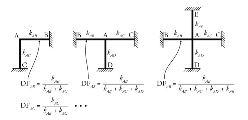
If the total rotational stiffness of a node is equal to the sum of the rotational stiffness of each element connected to that node, then the distribution factor for each member at the node is equal to the stiffness of that individual member divided by the total rotational stiffness of all the members connected to that node:
\begin{equation} \boxed{ \text{DF}_{AB} = \frac{k_{AB}}{\sum k_i} } \label{eq:stiff-dist} \tag{16} \end{equation}
where $\text{DF}_{AB}$ is the distribution factor for member AB at node A, $k_{AB}$ is the rotational stiffness of member AB for a moment applied at point A, and $\sum k_i$ is the sum of all the rotational stiffness values for all of the members connected to node A (including the one that we are calculating the distribution factor for). This process is illustrated in Figure 10.4.
All of the distribution factors for the members at a single joint must add up to $1.0$ because all of the moment must be divided up into the connected members. This is a good check to make sure that all the moment at a joint is accounted for.
The distribution factor for a fixed end support will be zero, and the distribution factor for a pin with only one member connected would be $1.0$.