 Learn About Structures
The moment distribution method for beams may be summarized as follows:
- Determine the stiffness for each member. For a member that is fixed at both ends, use equation \eqref{eq:stiff-fix}. \begin{equation} \boxed{ k_{AB} = \frac{4EI}{L} } \label{eq:stiff-fix} \tag{1} \end{equation} For a member that has a pin at one end, use equation \eqref{eq:stiff-pin}. \begin{equation} \boxed{ k_{AB} = \frac{3EI}{L} } \label{eq:stiff-pin} \tag{2} \end{equation}
- Determine the distribution factors for each member at each node based on relative stiffness of the members using equation \eqref{eq:stiff-dist}. \begin{equation} \boxed{ \text{DF}_{AB} = \frac{k_{AB}}{\sum k_i} } \label{eq:stiff-dist} \tag{3} \end{equation} Use a distribution factor of zero for a fixed support and 1.0 for a pinned support with only one connected member.
- Determine the fixed end moments for all members that have external loads applied between the end nodes. Use Figure 9.6 from Chapter 9.
- For each node in turn:
- Determine the unbalanced moment on the node.
- Distribute the unbalanced moment to each member connected to the node in proportion to the distribution factors in the reverse direction of the unbalanced moment.
- For each member that the moment has been distributed to, carry over some of the moment to the opposite end of the member according to equations \eqref{eq:carry-over-fixed} \begin{equation} \boxed{ \text{CO} = \frac{1}{2} } \label{eq:carry-over-fixed} \tag{4} \end{equation} and \eqref{eq:carry-over-pinned}. \begin{equation} \boxed{ \text{CO} = 0 } \label{eq:carry-over-pinned} \tag{5} \end{equation} For a member with a fixed end opposite (a regular locked node), carry over half of the moment that was applied by the distribution. For a member with a pinned end opposite (where there are no other members connected to that pin) do not carry over any moment.
- Repeat the previous step for each node, multiple times as necessary until the carry over moments are a small fraction of the total moments at each member end.
- Sum all of the moments in each member end from all previous steps (including the original fixed end moments). This sum gives the total moment at each member end in the real system.
Typically it is convenient to keep track of the iterative part of the above method using a table.
Example
The moment distribution method for beams will be illustrated in detail using the relatively simple example structure shown in Figure 10.5.

First, we need to find the stiffness of each member. Member AB has moment resistance at both ends, so we will use equation \eqref{eq:stiff-fix}:
\begin{align*} k_{AB} &= \frac{4EI}{L} \\ k_{AB} &= \frac{4EI}{5} \\ k_{AB} &= 0.8EI \end{align*}
Member BC has a pin at the right side node C with only one member (BC) connected to that node. So, for this member, we will find the stiffness using equation \eqref{eq:stiff-pin}:
\begin{align*} k_{BC} &= \frac{3EI}{L} \\ k_{BC} &= \frac{3EI}{4} \\ k_{BC} &= 0.75EI \end{align*}
The stiffness for both members is shown in Figure 10.6 part (a).
Next, we need to find all of the distribution factors for all the members at each joint. Let's first look at member AB at node A. If we consider the rotational stiffness of the fixed support at A to be infinite (it cannot rotate), then we can find the stiffness of member AB at node A as follows:
\begin{align*} \text{DF}_{AB} &= \frac{k_{AB}}{k_{AB} + k_{wall}} \\ \text{DF}_{AB} &= \frac{0.8EI}{0.8EI + \infty} \\ \text{DF}_{AB} &= 0 \end{align*}
This is an example that shows why we consider the distribution factor at a fixed support to be zero. Any moment that is carried over to the fixed support at A will stay there and never be distributed back into any other members. Even if we try to unlock the fixity at node A in our analysis, we cannot distribute the moment at the fixed support into any connected members. We do not have to unlock and redistribute forces at fixed support locations.
At node B there are two members that are connected, members AB and BC, both of which need distribution factors for node B:
\begin{align*} \text{DF}_{BA} &= \frac{k_{AB}}{k_{AB} + k_{BC}} \\ \text{DF}_{BA} &= \frac{0.8EI}{0.8EI + 0.75EI} \\ \text{DF}_{BA} &= 0.516 \\ \text{DF}_{BC} &= \frac{k_{BC}}{k_{AB} + k_{BC}} \\ \text{DF}_{BC} &= \frac{0.75EI}{0.8EI + 0.75EI} \\ \text{DF}_{BC} &= 0.484 \end{align*}
Notice that $\text{DF}_{BA} + \text{DF}_{BC} = 1.0$ as expected (all of the moment at the node must be distributed to the connected members).
For the pin end at node C, there is only one member attached, member BC:
\begin{align*} \text{DF}_{CB} &= \frac{k_{BC}}{k_{BC}} \\ \text{DF}_{CB} &= 1.0 \end{align*}
Since the pin cannot resist any moment, when the pin is unlocked, all of the moment must be distributed back to the single connected member. Since the distributed moment is equal to the negative of the unbalanced moment, the sum of the two will equal zero.
The next step is to determine the fixed end moments. Figure 9.6 was used to calculate the fixed end moments at either end of member BC as shown in Figure 10.6 part (b). These moments are equal to:
\begin{align*} \text{FEM}_{BC} = +25\mathrm{\,kNm} \\ \text{FEM}_{CB} = -25\mathrm{\,kNm} \end{align*}
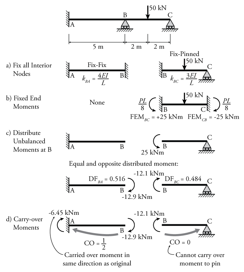
Now we have all of the information that we need to conduct the iterative moment distribution analysis. The moment distribution analysis is best kept track of using a table. For this example, the moment distribution analysis is shown in Table 10.1. The steps in this table up to the first carry over row are simultaneously depicted in Figure 10.6.
Table 10.1 begins at the top with a heading for each node. It may also be useful to label the nodes that are at fixed support locations (node A in this case), or pinned support conditions with no moment (node C in this case). Then, for each node, we need a column for every member that is connected to that node. In this example, nodes A and C only have one member each, and node B is connected to both members. It is also convenient to write the distribution factor for each member at each node underneath the member heading. We previously calculated the distribution factors for all members at all nodes based on the relative stiffness of each member at the node.
As previously discussed, we will start the analysis by assuming that all of the nodes are fixed for rotation. The next step is to apply the fixed end moments that we previously calculated to the appropriate member ends as shown in Table 10.1. This step is also shown in Figure 10.6 part (b). In this step, we must be careful about making sure that the sign of the moment is correct. Recall that counter-clockwise point moments are considered negative and clockwise moments are considered positive. These fixed end moments create unbalanced moments at nodes B and C. These unbalanced moments are held in place by the rotational fixity that we applied to each node at the beginning of the problem. At node B, for example, if we were to release the fixity, there is a moment of $+25\mathrm{\,kNm}$ on the node and no resisting moment in the opposite rotational direction, meaning that the node is not in equilibrium (which it must be for the node to be stationary.
So, if we were to release the rotational fixity at node B or C, the node would rotate due to the unbalanced moment, applying moments to all members connected to the joint, until the moments applied to the other members are in balance (in equilibrium). For this moment distribution analysis, we can start with either node B or C. We will start with node B.
So the next step is to release the rotational fixity at node B and rebalance the moments. This step is shown in Table 10.1 in the first row labelled 'Balance B' and simultaneously in Figure 10.6 part (c). To counteract the total unbalanced moment at node B of $+25\mathrm{\,kNm}$ we need to allow the node to rotate until a total counteracting moment of $-25\mathrm{\,kNm}$ is achieved by all of the members connected to the joint. Together, the original unbalanced moment of $+25\mathrm{\,kNm}$ and the new moment of $-25\mathrm{\,kNm}$ will add together to equal zero moment, meaning that node B attains equilibrium. The total counteracting moment of $-25\mathrm{\,kNm}$ is split between all of the connected members at node B according to their relative stiffness. This is the purpose of the distribution factors that we copied in at the top of the table. These distribution factors that we previously calculated tell us what percentage of moment goes in to each connected member. In this case the counteracting end moment in member BA is $0.516(-25) = -12.9$ and in member BC is $0.484(-25)=-12.1$. These must add up to the full counteracting moment value of $-25$. Once we apply the counteracting moment, it may be convenient to draw a line under them in the table as shown. This is an indication that all of the moments above the line are in equilibrium (they all add up to zero). This will help when calculating any new unbalanced moments that get applied to the node in the future.
Of course when we apply a moment to one end of a member, this may effect the value of the moment at the other end of the member. This is only true if we know that the other end of the member has some moment resistance (i.e. it is not a pin with only one member connected to it). This moment that is induced at the other end of the member is the carry-over moment. After balancing node B, the new counteracting moments which put the node into equilibrium when it is unlocked and balanced must be carried over to the other ends of all members connected to node B. Previously we found that applying a moment to one end of a member when the other end is fixed will result in half of that applied moment being induced at the opposite end of the member (in the same direction). So the counter balancing moment on member AB at node B of $-(-12.9\mathrm{\,kNm})$ ($M_{BA}$) will cause half of that moment at the other end of member AB at node A ($M_{AB} = -(-6.45\mathrm{\,kNm})$). This is the same as saying that the carry-over factor for that member $CO = \frac{1}{2}$. This carry-over is shown in Table 10.1 between BA and AB. For the other member connected to node B, member BC, the opposite end at node C is a pin that cannot take any moment. Therefore, the carry-over factor for that member $CO = 0$ as shown in the table. This carry-over process is also shown for the two members in Figure 10.6 part (d).
After node B is balanced and the carry-overs are applied to the opposite ends of the connected members, we re-lock (fix) node B and move onto another node in the structure. The order that we go in does not matter, but it is typically a good idea to go in some consistent order to ensure that all nodes are balanced, multiple times if necessary. In our case, we do not need to ever balance node A since it has a fixed support in the real structure. Any moments that are applied or carried over to the fixed support at node A will stay there permanently (the distribution factor for node A is 0).
So, we will move onto node C as shown in Table 10.1. The first step again is to unlock/release the node and balance the unbalanced moment. At node C, there is only one previous unbalanced load which was caused by the fixed end moment ($-25\mathrm{\,kNm}$); however, if there was a non-zero carry-over moment from the balancing of node B, then the total unbalanced moment for node C would be the sum of the original fixed end moment and the carried-over moment. The total counterbalancing moment for the unbalanced moment at node C is, therefore, $+25\mathrm{\,kNm}$ which is applied entirely to member CB (since it is the only member at the node and the distribution factor is 1.0). Since all the moments at node C are now balanced, there is a horizontal line drawn underneath the counterbalancing moment. Then, since the opposite end of that member, at node B, is fixed, we need to carry over half of the counterbalancing moment to the other end of member BC at node B ($+12.5\mathrm{\,kNm}$), as shown in the table.
So now, this has caused a new unbalanced moment at node B which needs to be balanced out again as shown in Table 10.1 (the second row that is labelled 'Balance B'). Since the carry-over moments from this balancing do not get transferred to the pin end at node C, there are no longer any unbalanced moments in the system after this step, so we are done with balancing nodes. It is not typical that a moment distribution analysis ends with perfectly balanced nodes as we will see in a later example. Typically, we need to keep iterating back and forth between nodes until the carry-over moments become sufficiently small as to be negligible.
The last step is to sum all of the moments that have been applied to each member end over the entire history of the analysis. Since we have used a table for our analysis (Table 10.1), we can just sum up all of the moment values in each column (each column representing one member end. This step is shown in the last row of the table, and these values give us the real moments are each end of each member.
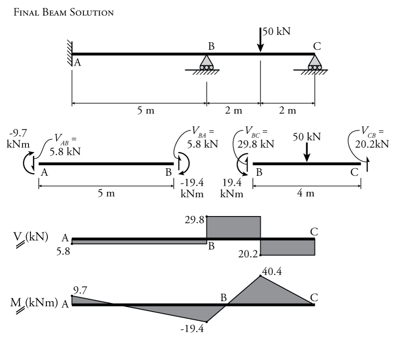
Using these moments, we can find the shears in the members and then draw the shear and moment diagrams for the beam as shown in Figure 10.7.