 Learn About Structures
The force method may also be used to determine the effect of support settlement, temperature changes and fabrication errors on indeterminate structures. The latter two will only be discussed in terms of their effect on indeterminate structures; we previously discussed and analysed their effect on determinate structures in Section 5.7.
Support Settlements
Support settlements may be caused by soil erosion, dynamic soil effects during earthquakes, or by partial failure or settlement of supporting structural elements. Supports could also potentially heave due to frost effects (this could be considered a negative settlement).
For externally determinate structures, support settlements will simply cause a rigid body rotation of the structure. Although this movement may be undesirable, the settlement cannot cause any internal forces in the structure itself. This situation is shown at the top of Figure 8.23. On the other hand, for indeterminate structures, settlement of structural supports can induce internal shears and moments as shown in the middle of Figure 8.23. This is because an indeterminate structure is effectively over-constrained, i.e. there are more restraints than the minimum required for stability.
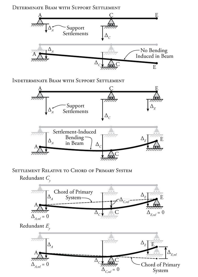
In Figure 8.23 an indeterminate beam is shown that has some support settlement at all three vertical support locations. It seems that the middle support at point C settles rather more than the others. So, this support effectively pulls down on the beam at point C, inducing bending in the beam. Now, of course, since all of the supports are settling to some extent in this example, the support at point C is not pulling down on the beam with a full effective displacement of $\Delta_C$ relative to the other two supports. It is only the portion of this settlement relative to the other two supports that causes bending in the beam.
We can think of this in terms of a determinate beam with the same geometry as the beam in Figure 8.23 but with supports only at points A and E. Imaging that there is now some action or load at point C that pulls the beam down at that location, causing bending in the beam. The determinate beam is not affected by the settlement of its supports at A and C, since support settlements do not cause moments in determinate beams as shown at the top of Figure 8.23. Instead, we would like to know how much point C moves down, relative to the determinate beam that can rotate freely as a rigid body as A and E settle. We can figure this out by drawing a straight line between points A and E (our determinate beam's undeflected shape) and then finding how far support C settles relative to that line.
This is a convenient way to think about things, especially when we are doing a force method analysis. In the force method, we already have a way to temporarily convert an indeterminate system into a determinate system for analysis by considering some of the forces as redundant. The determinate system that remains after we remove the restraints associated with the redundant forces is our primary system.
So, if we now consider the vertical reaction at point C ($C_y$)to be our redundant force (as shown in Figure 8.23), then we can consider our remaining primary system (with supports at A and E) as the determinate system that moves as a rigid body when its supports settle. We can then draw the chord of the primary system, which is just a straight line between points A and E (after they have settled). This chord represents the undeformed shape of the settled determinate primary system. Then, we can find how much the redundant support C has settled relative to the determinate system ($\Delta_{C,rel}$). This is the amount of deformation at point C which will cause the beam to bend and deflect.
To consider this relative imposed displacement caused by the support settlement at point C using the force method, all we have to do is modify our compatibility condition. Previously, all of our compatibility conditions typically equated to zero, since we were taking advantage of the compatibility information that a support doesn't move, or that the slope of a member is continuous at a point. For example, for a typical force method analysis where a vertical reaction at C was used as the redundant force, the compatibility condition may have looked something like:
\begin{align*} \Delta_{C0} + f_{CC} C_y = 0 \end{align*}
where $\Delta_{C0}$ is the deflection of the primary system at point C due to the external loads, $f_{CC}$ is the deflection of the primary system at point C due to a unit redundant load in that location (in the same direction as the reaction component), and $C_y$ is the reaction component at point C that we are trying to find. The right side of the equation is zero because we know that, typically, a vertical support remains stationary and holds the beam to zero displacement at the support location (i.e. in the real system $\Delta_C = 0$); however, if we now know that a support does not remain at zero, but actually settles by some known amount, then our compatibility condition will become:
\begin{align} \Delta_{C0} + f_{CC} C_y = \Delta_{C,rel} \tag{1} \end{align}
where $\Delta_{C,rel}$ is the relative settlement of the reaction at point C relative to the chord of the primary system (as shown in Figure 8.23). For the example shown in Figure 8.23, if the unit redundant force at point C is assumed to point up, then the magnitude of $\Delta_{C,rel}$ will be negative, because it settles downward relative to the chord of the primary system. To solve this type of problem, we would have to know the actual magnitude of the settlement at all of the support locations.
For the example in Figure 8.23, even though the support settlement is greatest at point C, it does not mean that we must select the reaction at point C as the redundant force for the force method analysis. The diagram at the bottom of the figure shows what would happen if we chose the reaction at point E as the redundant instead. In this case, the primary system is a determinate beam with supports at A and C. This means that the chord of the primary system is a straight line that runs right through these two points as shown. Now, even though the overall settlement of point E was downwards, relative to the chord of the primary system, the support at point E actually pushes the right end of the determinate primary beam up. The resulting compatibility condition for the force method analysis will be:
\begin{align} \Delta_{E0} + f_{EE} E_y = \Delta_{E,rel} \tag{2} \end{align}
but this time if the unit redundant is assumed to point up, then the magnitude of $\Delta_{E,rel}$ will be positive, because the beam heaves up at point E relative to the primary system.
This method also works with force method analyses for structures that are indeterminate to multiple degrees (that have multiple redundant forces). Two different example structures are shown in Figure 8.24. The structure shown at the top of that figure is a ${2^\circ}$ indeterminate propped cantilever and the structure shown at the bottom is a ${2^\circ}$ indeterminate multi-span beam.
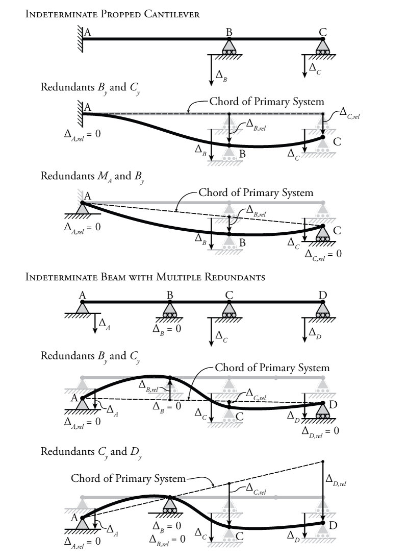
For the indeterminate propped cantilever in Figure 8.24, there are two different sets of possible redundant forces shown. If the vertical reactions at points B and C ($B_y$ and $C_y$) are used as the redundant forces, then the primary system is a simple cantilever with a fixed end at point A. So the chord of the primary system is simply a horizontal line that follows the undeformed shape of the structure. In this case the relative settlements of supports B and C are simply equal to the full settlement magnitude ($\Delta_{B,rel} = \Delta_B$ and $\Delta_{C,rel} = \Delta_C$). The compatibility conditions for this analysis will be:
\begin{align} \Delta_{B0} + f_{BB} B_y + f_{BC} C_y &= \Delta_{B,rel} \tag{3} \\ \Delta_{C0} + f_{CB} B_y + f_{CC} C_y &= \Delta_{C,rel} \tag{4} \end{align}
Since no external loads are provided for this example, $\Delta_{B0}$ and $\Delta_{C0}$ would be equal to zero. If the moment reaction at point A and the vertical reaction at point B ($M_A$ and $B_y$) are used as the redundant forces, then the resulting determinate primary system is a simply supported beam between points A and C. This beam experiences a rigid body rotation due to the support settlement at point C, resulting in the chord for the primary system shown in Figure 8.24. Using the geometry of the system, we must then find the value of $\Delta_{B,rel}$ based on the location of the chord at point B. The compatibility conditions for this analysis will be:
\begin{align} \theta_{A0} + f_{AA} M_A + f_{AB} B_y &= 0 \tag{5} \\ \Delta_{B0} + f_{BA} M_A + f_{BB} B_y &= \Delta_{B,rel} \tag{6} \end{align}
Again, since no external loads are provided for this example, $\theta_{A0}$ and $\Delta_{B0}$ would be equal to zero. Note that the right side of the first compatibility equation is still zero, because the rotation of the full system at point A is still known to be zero.
For the indeterminate multi-span beam shown in the lower half of Figure 8.24, two different combinations of redundants are shown along with their associated primary systems, and the chords of those primary systems. This example shows that, depending on the selection of your redundant forces, even supports that do not have any absolute support settlement may have a displacement relative to the chord of the primary system.
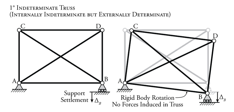
Support settlement only affects structures that are externally indeterminate. Structures that are internally indeterminate but externally determinate will not experience any induced internal forces caused by support settlement. An example of such a structure is shown in Figure 8.25. The internally indeterminate truss is externally determine because it only has three reaction components. If one of the supports settles, the truss will only experience a rigid body rotation, but no extra internal axial forces.
Example
The use of the force method to analyse a beam structure with a support settlement will be illustrated using the example structure shown in Figure 8.26. This structure is a two span beam with a roller support at the right end that settles downwards by $45\mathrm{\,mm}$. Note that, even though $EI$ is constant for the whole beam in this example, we still need to know the values of $E$ and $I$ if we want to find the internal bending moments cause by the support settlement. The higher the stiffness of the beam, the higher the induced moments caused by the support settlement will be.
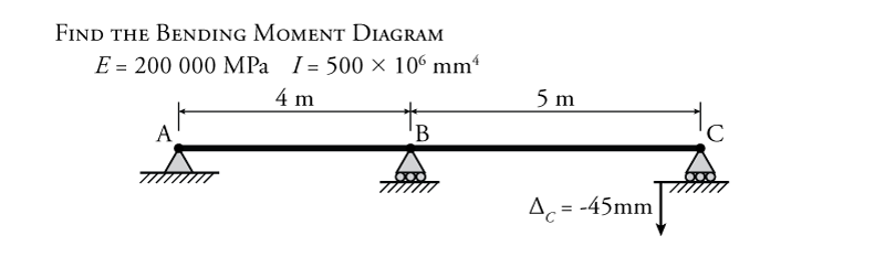
Even though the settlement happens at point C in this example, the vertical reaction force at point C ($C_y$) may not be the best choice for the redundant force because the resulting primary system will be a beam with an overhang, which may not be the easiest structure to analyse. A better choice for a redundant would be the vertical reaction force at point B ($B_y$) since the resulting primary system will be a simply supported beam, which will be easier to analyse. The resulting primary system is shown in Figure 8.27.
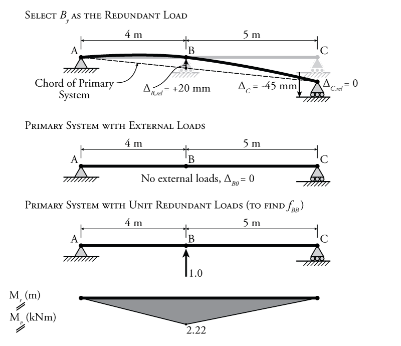
The primary system resulting from the redundant load $B_y$ has an associated chord that is also shown in Figure 8.27. The primary system is not horizontal due to the support settlement at point C. We know that point B does not settle ($\Delta_B = 0$, but since the chord of the primary system is not horizontal, the redundant support at point B does have a displacement relative to the chord of the primary system, as shown. We can calculate this from geometry. In this case, we need to first find the vertical location of the chord at the horizontal location along the beam associated with point B:
\begin{align*} \Delta_{Chord,B} &= \frac{4}{9} (\Delta_C) \\ \Delta_{Chord,B} &= \frac{4}{9} (-45) \\ \Delta_{Chord,B} &= -20\mathrm{\,mm} \end{align*}
So, to get to the stationary point B from the chord of the primary system, you would have to push up by $20\mathrm{\,mm}$, so:
\begin{align*} \Delta_{B,rel} = +20\mathrm{\,mm} \end{align*}
Now, we can define our compatibility condition for the restraint associated with the redundant force $B_y$:
\begin{align*} \Delta_{B0} + f_{BB} B_y = \Delta_{B,rel} \end{align*}
+Since there is no external load in this problem, $\Delta_{B0} = 0$ as shown in Figure 8.27. So the completed compatibility condition is:
\begin{align*} f_{BB} B_y = 20\mathrm{\,mm} \end{align*}
From this point forward, the analysis is the same as any other force method analysis. The only unknown that is left in our compatibility equation (since $\Delta_{B0}$ is zero), is the flexibility coefficient $f_{BB}$. To find $f_{BB}$, we can use virtual work to find the effect of a unit redundant load at point B on the deflection of the beam at point B. For this analysis, the real and virtual moment diagrams will be the same as shown at the bottom of Figure 8.27, except that the units for those diagrams are different since the unit redundant force is unitless. Applying virtual work using the product integration table from Figure 5.22:
\begin{align*} W_{v,i} &= \frac{1}{EI} \left( \frac{LMQ}{3} \right) + \frac{1}{EI} \left( \frac{LMQ}{3} \right)\\ W_{v,i} &= \frac{(4)(2.22)(2.22)}{3EI} + \frac{(5)(2.22)(2.22)}{3EI} \\ W_{v,i} &= \frac{14.81\mathrm{\,kN m^3}}{EI} \end{align*}
Applying the virtual work balance:
\begin{align*} W_{v,e} &= W_{v,i} \\ (1\mathrm{\,kN})(f_{BB}) &= \frac{14.81\mathrm{\,kN m^3}}{EI} \\ f_{BB} &= \frac{14.81\mathrm{\,m^3}}{EI} \end{align*}
Knowing the flexibility coefficient $f_{BB}$, we can now solve for the unknown redundant force $B_y$ using the compatibility condition:
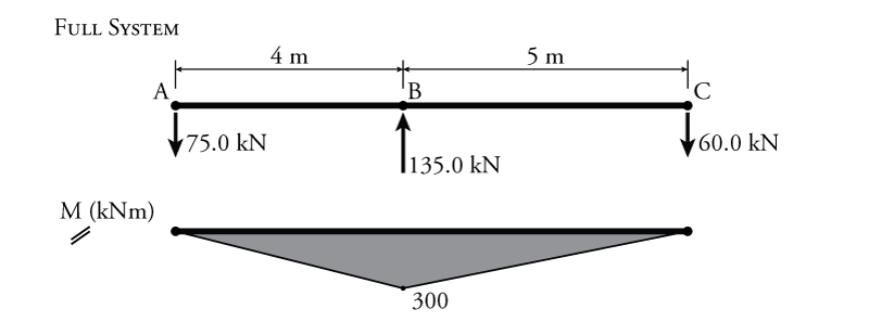
\begin{align*} f_{BB} B_y &= 20\mathrm{\,mm} \\ B_y &= \frac{ 20\mathrm{\,mm} (EI) }{ 14.81\mathrm{\,m^3} } \\ B_y &= \frac{ 20\mathrm{\,mm} (200000\mathrm{\,MPa}) (500\times 10^6\mathrm{\,mm^4}) }{ 14.81\times 10^9\mathrm{\,mm^3} } \\ B_y &= 135.0\mathrm{\,kN} \uparrow \end{align*}
Knowing this single reaction reduces the number of unknown reaction components in the indeterminate system from four to three, meaning that the rest may be found using equilibrium as shown in Figure 8.28. Then, the final moment diagram for the indeterminate structure may also be drawn as shown in the figure. Since there were no external forces on this sample beam, this internal bending moment was created solely by the settlement of support C.
Temperature Changes and Fabrication Errors in Trusses
Temperature changes and fabrication errors will affect all kinds of indeterminate structures; however, in this course, we will only look at their effect on indeterminate trusses.
To analyse an indeterminate truss with a temperature change or fabrication error, we must simply conduct the force method analysis as usual, except that the external 'loadings' on the primary system may derive from the temperature change or fabrication error. We previously studied the effect of temperature changes and fabrication errors on determinate trusses using virtual work. This was discussed in Section 5.6. Since the primary system in a force method analysis is determinate, the same analysis methods apply here.
Although these temperature and fabrication effects do change the internal forces in the indeterminate structure, in the determinate primary structure, they have no effect on the internal axial forces, they only effect the deformations, which we will then use within the appropriate compatibility condition.
Example
This process will be illustrated using the sample indeterminate truss shown in Figure 8.29. This truss has one member affected by a local temperature change (member CD) and one member that was fabricated too long (member BD). Although there are no external forces on the truss, these two effects will cause internal axial forces since the truss is indeterminate. Note also that the two diagonal members in the truss cross in the middle but are not connected at that point. Both diagonal members are only connected to the outside corners of the truss.
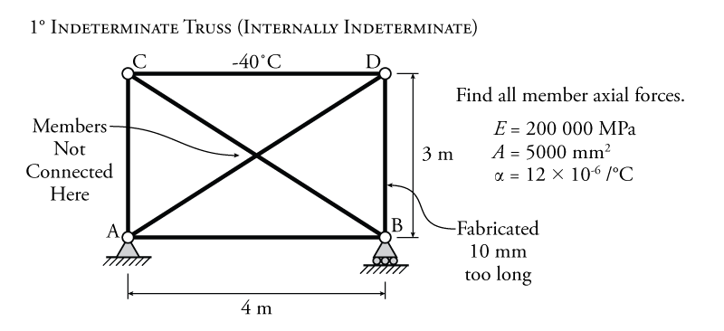
The first step, as for all previous force method analyses is to choose a redundant force. This truss is internally indeterminate but externally determinate. Therefore, we must select an internal force as the redundant force (as described previously in Section 8.3). For this example, we will use the internal axial force in truss member BC as the redundant force. Therefore, we must break member BC for axial force to form our primary system as shown at the top of Figure 8.30. As before, the compatibility condition for this force method analysis is:
\begin{align*} \Delta_{BC,0} + f_{BCBC} F_{BC} = 0 \end{align*}
where $\Delta_{BC,0}$ is the overlap or gap between the cut section ends b and c caused by the external forces, $f_{BCBC}$ is the overlap or gap between the cut section ends b and c caused by the pair of unit redundant forces at the cut ends, and $F_{BC}$ is the magnitude of the redundant force (which we are trying to solve for).
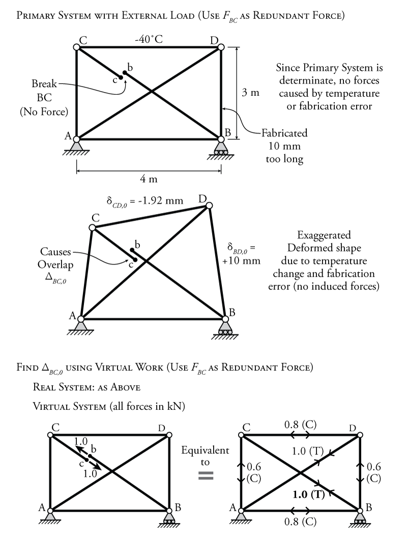
The next step is to apply our external forces to the primary system and determine the overlap at the break location in Member BC ($\Delta_{BC,0}$). The only external 'forces' that we have in this problem are the local temperature change on member CD and the fabrication error for member BD. These effects both result in member deformations for those members. For the temperature change:
\begin{align*} \delta_{CD,0} &= \alpha (\Delta T) L \\ \delta_{CD,0} &= (12\times 10^{-6}\mathrm{\,/ ^\circ C}) (-40\mathrm{\,^\circ C}) (4000\mathrm{\,mm}) \\ \delta_{CD,0} &= -1.92\mathrm{\,mm} \end{align*}
For the fabrication error, the deformation is directly equal to the error amount:
\begin{align*} \delta_{DB,0} = +10\mathrm{\,mm} \end{align*}
These effects do not cause axial force in the primary system, since it is determinate. An exaggerated deformed shape for the truss is shown in Figure 8.30. To find the overlap $\Delta_{BC,0}$, we can use virtual work. The real system for this virtual work analysis is the determinate primary system with the temperature and fabrication effects accounted for. The virtual system is the primary system with virtual external unit loads at the cut ends of member BC (at points b and c) as shown at the bottom of Figure 8.30.
As discussed in Section 8.3, the virtual system with unit virtual external unit loads at the cut ends is equivalent to a truss with a diagonal member BC that has an axial tension of $1\mathrm{\,kN}$ as shown at the bottom of Figure 8.30. The calculation of the resulting internal virtual work analysis to find the unknown overlap $\Delta_{BC,0}$ is shown in Table 8.3.
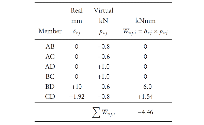
Applying the virtual work balance:
\begin{align*} W_{v,e} &= W_{v,i} \\ (1\mathrm{\,kN})(\Delta_{BC,0}) &= -4.46\mathrm{\,kN mm} \\ \Delta_{BC,0} &= -4.46\mathrm{\,mm} \end{align*}
The next step is to find the flexibility coefficient $f_{BCBC}$ which is the overlap at the cut section in the primary system caused by a pair of unit redundant forces applied to either cut end. For this part of the analysis, using virtual work, the real and virtual systems are both the same as the virtual system for the external load analysis shown at the bottom of Figure 8.27. The solution for this flexibility coefficient is the same as for the example problem from Section 8.3. The calculation for the internal virtual work is the same as previously shown in Table 8.2, which resulted in a flexibility coefficient of:
\begin{align*} f_{BCBC} &= \frac{17.28\mathrm{\,m}}{EA} \end{align*}
Now that we have solved for $\Delta_{BC,0}$ and $f_{BCBC}$, we can use the compatibility equation for the system to solve for the redundant force magnitude $F_{BC}$:
\begin{align*} \Delta_{BC,0} + f_{BCBC} F_{BC} &= 0 \\ F_{BC} &= -\frac{\Delta_{BC,0}}{f_{BCBC}} \\ F_{BC} &= - \left( -4.46\mathrm{\,mm} \right) \left( \frac{EA}{17.28\mathrm{\,m}} \right)\\ F_{BC} &= - \left( -4.46\mathrm{\,mm} \right) \left( \frac{(200000\mathrm{\,MPa})(5000\mathrm{\,mm^2})}{17.28\mathrm{\,m}} \right)\\ F_{BC} &= - \left( -4.46\mathrm{\,mm} \right) \left( \frac{(200000\mathrm{\,MPa})(5000\mathrm{\,mm^2})}{17280\mathrm{\,mm}} \right)\\ F_{BC} &= +258\mathrm{\,kN} \\ F_{BC} &= 258\mathrm{\,kN} \; \text{(Tension)} \end{align*}
Going back to the full system now, with the redundant force in member BC included in the truss as a known force, the rest of the truss member axial forces may be found. This complete truss solution is shown in Figure 8.31.
