 Learn About Structures
The Bernoulli-Euler beam theory (Euler pronounced 'oiler') is a model of how beams behave under axial forces and bending. It was developed around 1750 and is still the method that we most often use to analyse the behaviour of bending elements. This model is the basis for all of the analyses that will be covered in this book.
The Bernoulli-Euler beam theory relies on a couple major assumptions. Of course, there are other more complex models that exist (such as the Timoshenko beam theory); however, the Bernoulli-Euler assumptions typically provide answers that are 'good enough' for design in most cases.
Bernoulli-Euler Assumptions
The two primary assumptions made by the Bernoulli-Euler beam theory are that 'plane sections remain plane' and that deformed beam angles (slopes) are small.
The plane sections remain plane assumption is illustrated in Figure 5.1. It assumes that any section of a beam (i.e. a cut through the beam at some point along its length) that was a flat plane before the beam deforms will remain a flat plane after the beam deforms (i.e. it will not curve out-of-its-own-plane as shown in the lower right image within Figure 5.1). This assumption is generally relatively valid for bending beams unless the beam experiences significant shear or torsional stresses relative to the bending (axial) stresses. Shear stresses in beams may become large relative to the bending stresses in cases where a beam is very deep and short in length.
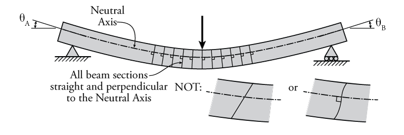
The plane sections remain plane assumption also assumes that any section of a beam that was perpendicular to the neutral axis before the beam deforms will remain perpendicular to the neutral axis after the beam deforms. Recall that, depending on the cross-sectional shape of the beam and its composition, the neutral axis may not be located at the mid-height of the beam.
Secondly, if we can assume that the deformed angles (slopes) of the beam are small (represented by $\theta$ in Figure 5.1), then there are some significant benefits to the analysis. If $x$ represents the location along the length of the beam, and $\Delta(x)$ is the displacement of the beam at location $x$, then the slope ($\theta$) of the beam is:
\begin{equation} \tag{1} \theta = \frac{d\Delta}{dx} \end{equation}
+which is simply the change in $\Delta$ with respect to $x$ (you can also think of this as rise over run). If the slope $\theta$ is small, then it stands to reason that the square of the slope would be doubly small and can assumed to be equal to zero:
\begin{equation} \tag{2} \theta^2=\left( \frac{d\Delta}{dx} \right) ^2 \approx 0 \end{equation}
+In addition, for small angles, the following approximations are also valid (as demonstrated in Table 5.1):
\begin{align} \tag{3} \sin \theta \approx \theta \\ \tag{4} \cos \theta \approx 1 \end{align}
+if $\theta$ is the slope in radians. As the table shows, up to ${5^\circ}$, these approximations are almost exact to three significant figures. At ${10^\circ}$, there may be up to $1.5\%$ error.
| Angle $\theta$ (deg.) | Angle $\theta$ (rad.) | $\sin \theta$ | $\cos \theta$ |
|---|---|---|---|
| $0$ | $0$ | $0$ | $1$ |
| $1$ | $0.0175$ | $0.0175$ | $0.9999$ |
| $2$ | $0.0349$ | $0.0349$ | $0.9994$ |
| $5$ | $0.0873$ | $0.0872$ | $0.996$ |
| $10$ | $0.175$ | $0.174$ | $0.985$ |
The Bernoulli-Euler Beam Equation
Based on the assumptions discussed above, the Bernoulli-Euler Beam Theory results in the following equation:
\begin{equation} \tag{5} \boxed{ \frac{d^2\Delta}{dx^2} = \frac{M}{EI} } \end{equation}
where $ \frac{d^2\Delta}{dx^2}$ is the second derivative of the deflection of the beam $\Delta$ with respect to the position along the beam $x$, $M$ is the internal moment in the beam at location $x$, $E$ is the Young's modulus of the beam material, and $I$ is the moment of inertia (second moment of area) of the beam cross-section. This differential equation applies for any point along the beam, as long as our assumptions (plane sections remain plane and small angles) remain reasonably valid. The derivation of this equation may be found elsewhere in other structural analysis texts.
For the purposes of this course, the following points about the Bernoulli-Euler beam equation are important to know and understand:
- Curvature is equal to the slope of the strain profile -- Curvature (symbol $\phi$) is a measure of how much bending deforming a beam has at a particular location (the intensity of the curve). One consequence of the "plane sections remain plane" assumption is that the strain profile is linear as shown in Figure 5.2. The slope of that linear strain profile with respect to the beam height is equal to the curvature of the beam at that point. For the situation shown in Figure 5.2, the slope of the strain profile (curvature) may be calculated as: \begin{equation*} \phi = \frac{\epsilon}{y} \end{equation*}
where $y$ is the distance to the top fibre from the neutral axis, and $\epsilon$ is the strain in that top fibre.
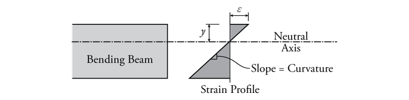 Figure 5.2: Definition of Curvature
 - The Radius of Curvature is the Inverse of the Curvature -- If the curve at a point on a bending beam was matched up against a circle that has the the same curvature, then the radius of that circle is the radius of curvature of the beam (symbol $R$). It can be calculated from the curvature by: \begin{equation} \tag{6} \boxed{R = \frac{1}{\phi}} \end{equation}
- Curvature is approximately equal to the second derivative of the deflection with respect to position: \begin{equation} \tag{7} \boxed {\phi = \frac{1}{R} \approx \frac{d^2\Delta}{dx^2}} \end{equation}
which is also equivalent to the change in slope with respect to position:
\begin{equation} \tag{8} \boxed {\phi = \frac{1}{R} \approx \frac{d\theta}{dx}} \end{equation} - Curvature is directly related to the moment: \begin{equation} \tag{9} \boxed{\phi = \frac{M}{EI} } \end{equation}
Therefore:
\begin{equation} \tag{10} \boxed {\frac{d^2\Delta}{dx^2} =\frac{d\theta}{dx} \approx \frac{M}{EI} } \label{eq:mom-curv} \end{equation}