 Learn About Structures
Virtual work for beams is different than for truss elements because beams can deform and store strain energy in multiple different ways. Like truss elements, beams can deform axially, but they can also bend and shear. As mentioned previously in Section 5.6, for beam bending problems, the deformations caused by axial force and shear force are typically insignificant in comparison to the deformations caused by bending. So, for beams, we can get a very good estimate of the deflections by considering only the internal virtual work done by bending moments.
In addition, beams have both deflections and rotations along their length, so we need to be able to solve for either of these. To solve for the deflection or rotation at some point on a beam, the unit virtual external force on a beam can be either a unit point load or a unit point moment. It still must be located at the location along the beam where we want to find the displacement/rotation and must be in the same direction as the displacement/rotation that we want to find. For example, for a vertical displacement, we must use a vertical virtual unit load, and for a clockwise rotation, we should use a clockwise point moment. The external virtual work for beams looks very similar to the external virtual work for trusses:
\begin{align*} \boxed{W_{v,e} = (1)(\Delta_r \, \text{or} \, \theta_r)} \end{align*}
where $(1)$ is the unit load or unit point moment, $\Delta_r$ is a real external displacement that we are trying to find (in the same location and direction as the unit point load), or $\theta_r$ is a real external rotation that we are trying to find (in the same location and direction as the unit point moment).
In contrast, the internal virtual work calculations are completely different for beams than they were for trusses. For truss members, we had to sum up discrete axial deformations and forces for each truss member. The internal real deformations were equal to the deformation of each truss element in the real system and the internal virtual forces were equal to the internal axial forces in each truss element in the virtual system. For a beam, since we are only considering work that is stored in the form of bending strains in the beam, the internal real deformations are equal to the beam rotations along the length of the beam in the real system, and the internal virtual forces are equal to the internal moment along the length of the beam in the virtual system.
Since we now have a continuous beam instead of discrete truss elements, we must look at the curvature and moment of infinitesimally small pieces of the beam and integrate them along the length to find the total internal virtual work. Recall that the internal virtual work is equal to:
\begin{equation*} W_{v,i} = \sum \left( \text{Virtual Int. Forces} \; \times \text{Real Int. Deformations} \right) \end{equation*}
For our continuous beam, we can look at the small increment of work that is added for each small piece of the beam:
\begin{align} dW_{v,i} = M_v (d \theta_r) \label{eq:virt-beam-dW} \tag{1} \end{align}
where $M_v$ is the virtual internal moment applied to that small piece and $d\theta_r$ is the real system change in slope from one side of the small piece to the other. Recall also from the Bernoulli-Euler Beam theory equation, that:
\begin{align} d\theta_r = \frac{M_r}{EI} dx \label{eq:virt-beam-dtheta} \tag{2} \end{align}
where $M_r$ is the real internal moment, $E$ is the Young's modulus of the material, $I$ is the moment of inertia of the beam cross section, and $x$ is the position along the length of the beam. Recall that $M_r/EI$ is equal to the curvature of the real beam $\phi_r$. Combining equations \eqref{eq:virt-beam-dW} and \eqref{eq:virt-beam-dtheta}, we get:
\begin{align} dW_{v,i} = M_v \frac{M_r}{EI} dx \tag{3}\end{align}
To find the total work over the entire length of the beam, we can integrate to get:
\begin{equation} \boxed{W_{v,i} = \int_0^L \frac{M_vM_r}{EI} dx} \label{eq:Virtual-Work-Internal-Beams} \tag{4} \end{equation}
where $L$ is the length of the beam. Note that in this equation, $M_v$, $M_r$, $E$ and $I$ may all potentially be functions of the position along the beam $x$. This equation may also be rewritten as:
\begin{equation} \boxed{W_{v,i} = \int_0^L M_v \phi_r dx} \tag{5} \end{equation}
Now that we have expressions for internal and external virtual work for beams, we can combine them together into a single virtual work balance:
\begin{align*} W_{v,e} = W_{v,i} \end{align*} \begin{equation} \boxed{(1)(\Delta_r \, \text{or} \, \theta_r) = \int_0^L \frac{M_vM_r}{EI} dx} \label{eq:Virtual-Work-Balance-Beams} \tag{6} \end{equation}
This seems like this will be a difficult solution because it requires integration of the product of the virtual moment diagram and the real curvature diagram (which it does). If we find the virtual moment and real curvature for the beam as a function of the position $x$, then we can simply plug those functions into equation \eqref{eq:Virtual-Work-Balance-Beams} and solve the integral. This is not too difficult because our functions for moment and curvature are typically polynomials; however, we can use tables of product integrals to make this process significantly easier.
A virtual work product integration table is shown in Figure 5.22. The virtual moment and real curvature diagrams may be split into simply-shaped pieces. Then the equations in the table can be used to find the the integral of the product of a curvature diagram piece multiplied by the moment diagram piece. When applying this table, the individual pieces must be for the same portion of the beam for both the virtual system and the real system (e.g. both pieces cover the beam between $x = 2\mathrm{\,m}$ and $x = 5\mathrm{\,m}$.

Example
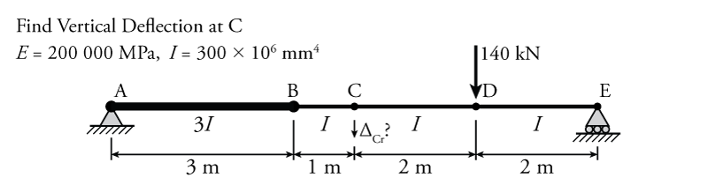
The use of the virtual work product integration table to calculate the total internal virtual work will be illustrated using the example beam shown in Figure 5.23. It is a simply supported beam with a stiff section on the left between A and B, and a point load at point D towards the right. Therefore, this example will also demonstrate the effect of a varying beam moment of inertia ($I$) on the curvature diagram.
The real and virtual systems for the example beam are shown in Figure 5.24, with the real system at the top and the virtual system at the bottom. The real system free body diagram is shown with the support reaction forces at either end. Below that, is the moment diagram of the real beam, which is not affected by the higher moment of inertia between points A and B. Below the real moment diagram is the real beam curvature diagram, which represents the real internal deformation for the calculation of the internal virtual work. This curvature diagram has a step up at point B. This step is due to the change in the moment of inertia of the beam cross section from $3I$ to $I$. The curvature values in the diagram are given as a function of $1/EI$. So, when $I$ triples, the curvature is divided by three. After the curvature diagram is constructed, it is divided into simple shapes that can be found in Figure 5.22 as shown by the varying shading in Figure 5.24. The real curvature diagram in the example is split into two triangles and two trapezoids, each shape being numbered '1' through '4.'
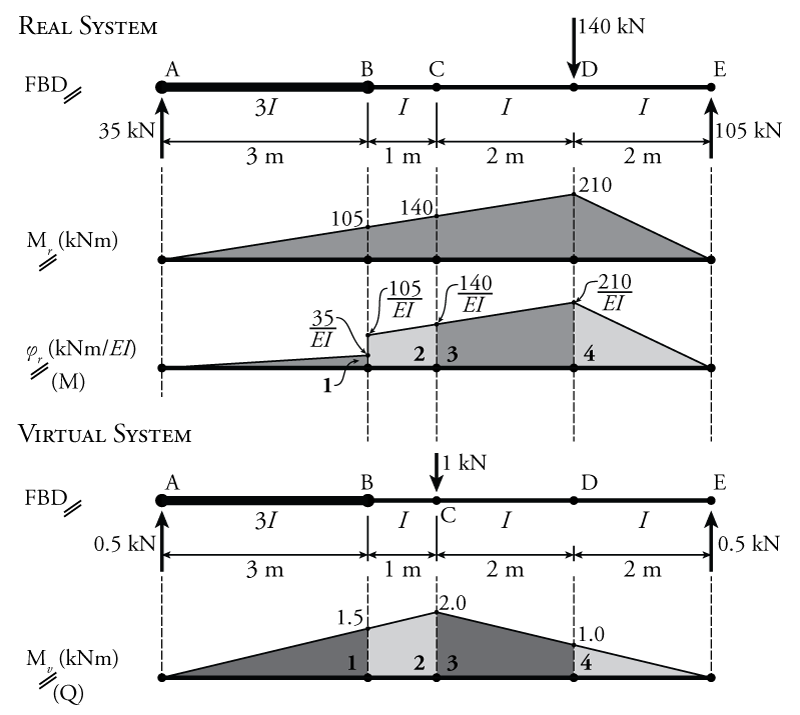
The lower half of Figure 5.24 shows the virtual system. Since we want to find the vertical deflection at point C, the virtual external unit load is placed at point C and directed vertically. The resulting free body diagram for that virtual system is shown, including the support reaction forces (which, as described previously, do not affect the external virtual work because the displacement of the support reactions must be zero).
Then, then moment diagram for the virtual system may be constructed as shown at the bottom of Figure 5.24. This moment diagram represents the virtual internal force. There is no need to calculate the curvature diagram for the virtual system because there is no need for virtual internal deformations in our virtual work balance.
The resulting virtual moment diagram is, in itself, a large triangle, which is a shape that can be found in Figure 5.22; however, when using the product integral expressions from Figure 5.22 find the total internal virtual work, the divided sections for the real and virtual systems must coincide. So, the virtual moment diagram must be divided up into equivalent sections to those from the real curvature diagram. These four sections for the virtual moment diagram are shown using shading and are numbered '1' to '4' to match each section from the real curvature diagram.
Once we have constructed the real curvature diagram and the virtual moment diagram, and subdivided them into simple shapes, we can use the product integrals from Figure 5.22 to calculate the total internal virtual work for the combined real-virtual system. This entails selecting the right expression from the figure for each section of the beam ('1' through '4'). When using Figure 5.22, the real curvature will typically be the 'M' system, and the virtual moment diagram will be the 'Q' system (as indicated in Figure 5.24)).
For section '1,' the real curvature diagram is a triangle and the virtual moment diagram is also a triangle. Looking at Figure 5.22, the integral for the product of a triangle and another triangle where the high side of both is on the same side is:
\begin{align*} \int_0^L M Q \, dx = \frac{LMQ}{3} \end{align*}
which is from the second row, second column, which, in our terms, is equivalent to:
\begin{align*} \int_0^3 \phi_r M_v \, dx &= \frac{1}{3} \left( 3 \right) \left( \frac{35}{EI} \right) \left( 1.5 \right) \\ &= \frac{52.5\mathrm{\,kN^2 m^3}}{EI} \end{align*}
which is the first term of our internal virtual work. The units of the numerator are $\mathrm{kN^2m^3}$ because we have a curvature (units $\mathrm{kNm/EI}$), multiplied by a moment (units $\mathrm{kNm}$), multiplied by a length (units $\mathrm{m}$). It is important to note that if the high side of the triangle for the real curvature was on the left and the high side of the triangle for the virtual moment was on the right, then a different equation from Figure 5.22 would apply (second row, third column $\frac{LMQ}{6}$).
For section '2,' the real curvature diagram is a trapezoid and the virtual moment diagram is also a trapezoid. Looking at Figure 5.22 again, the integral of the product of two trapezoids is:
\begin{align*} \int_0^L M Q \, dx = \frac{L}{6} \left[ Q_a (2M_a + M_b) + Q_b (M_a + 2M_b) \right] \end{align*}
from the fifth row, fourth column, which, in our terms, is equivalent to:
\begin{align*} \int_0^3 \phi_r M_v \, dx &= \frac{1}{6} \left[ 1.5 \left( 2 \left( \frac{105}{EI} \right) + \frac{140}{EI} \right) + 2.0 \left( \frac{105}{EI} + 2 \left( \frac{140}{EI} \right) \right) \right] \\ &= \frac{215.8\mathrm{\,kN^2 m^3}}{EI} \end{align*}
Continuing in this way for the rest of the sections:
\begin{align*} W_{v,i} &= \int \text{Section 1} + \int \text{Section 2} + \int \text{Section 3} + \int \text{Section 4} \\ &= \frac{1}{3} \left( 3 \right) \left( \frac{35}{EI} \right) \left( 1.5 \right) \\ & \;\; + \frac{1}{6} \left[ 1.5 \left( 2 \left( \frac{105}{EI} \right) + \frac{140}{EI} \right) + 2.0 \left( \frac{105}{EI} + 2 \left( \frac{140}{EI} \right) \right) \right] \\ & \;\; + \frac{2}{6} \left[ 2 \left( 2 \left( \frac{140}{EI} \right) + \frac{210}{EI} \right) + 1.0 \left( \frac{140}{EI} + 2 \left( \frac{210}{EI} \right) \right) \right] \\ & \;\; + \frac{1}{3} \left( 2 \right) \left( \frac{210}{EI} \right) \left( 1.0 \right) \\ &= \frac{52.5 + 215.8 + 513.3 + 140}{EI} \\ W_{v,i} &= \frac{921.6\mathrm{\,kN^2m^3}}{EI} \end{align*}
Since this is not the final answer yet, it's okay to keep a couple extra significant figures.
Now applying our virtual work balance:
\begin{align*} W_{v,e} &= W_{v,i} \\ (1\mathrm{\,kN}) (\Delta_{Cr}) &= \frac{921.6\mathrm{\,kN^2m^3}}{EI} \\ \Delta_{Cr} &= \frac{921.6\mathrm{\,kN^2m^3}}{(1\mathrm{\,kN}) (200000\mathrm{\,MPa}) (300\times 10^6\mathrm{\,mm^4})} \\ \Delta_{Cr} &= \frac{921.6\times 10^15\mathrm{\,N^2mm^3}}{(1000\mathrm{\,N}) (200000\mathrm{\,MPa}) (300\times 10^6\mathrm{\,mm^4})} \end{align*} \begin{equation} \boxed{\Delta_{Cr} = 15.4\mathrm{\,mm} \downarrow } \end{equation}
The deflection is downwards because our assumed virtual external unit force was assumed to point downward and the answer for $\Delta_{Cr}$ was positive. In the above expression, all of the units were converted into $\mathrm{N}$, $\mathrm{mm}$ and $\mathrm{MPa}$ first so that the answer would be in $\mathrm{mm}$ (recall that $1\mathrm{\,MPa}=1\mathrm{\,N/mm^2}$).